Determining Series RLC Circuit Resonance Frequency

A series RLC circuit contains a resistor (R), an inductor (L), and a capacitor (C) connected in series. Resonance in a series RLC circuit occurs when the reactive effects of the inductor and capacitor cancel each other out, resulting in a purely resistive circuit. At resonance, the circuit exhibits some interesting properties, such as a maximum current and a minimum impedance. Understanding the phenomenon of resonance in a series RLC circuit is essential in designing and analyzing many electronic devices and systems.

 

Frequency Effect on Circuit Impedance

The series-connected RLC circuit shown in Figure 1(a) has an impedance of

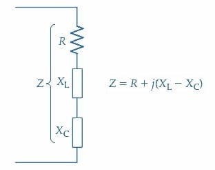
\[Z=R+j{\big(}X_{L}-X_{C}{\big)}\,(1)\]

Or

\[Z=\sqrt{R^{2}+X^{2}}\angle tan^{-1}{\Big(}\frac{X}{R}{\Big)}\]

Because X_L=2πfL and X_C=1/(2πfC), the actual impedance of the circuit depends on the frequency of the alternating supply, as illustrated in Figure 1(b). Figure 2 shows the values of jX_L and -jX_C plotted versus supply frequency. It is seen that because X_L is directly proportional to frequency, the inductive reactance increases linearly from zero with the increase in frequency. However, the capacitive reactance is inversely proportional to the frequency, and at low frequencies, X_C is infinitely large. As the frequency increases, X_C rapidly decreases from infinity but never becomes zero. The resulting graph of (-jX_C) versus frequency is curved, as illustrated.

 

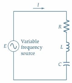
(a) Series RLC circuit with a variable frequency source.

 

(b) X_L and X_C vary with the frequency of the voltage source.

Figure 1. In a series RLC circuit with a variable frequency source, X_L becomes equal to X_C at a particular frequency, known as the resonance frequency. The circuit impedance is then equal to R. Image used courtesy of Amna Ahmad

 

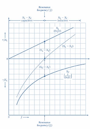
Figure 2. A plot of +jX_L and -jX_C versus frequency for a series RLC circuit shows that at a particular frequency (f_r), X_L = X_C, and consequently (X_L = X_C) = 0. The frequency f_r is known as the resonance frequency for the circuit. Image used courtesy of Amna Ahmad

 

The total reactance of the series-connected RLC circuit is (X_L - X_C), and the graph of this quantity is shown by the dashed line in Figure 2. At low frequencies, it is clear that X_L is much smaller than X_C, and thus the total reactance is largely capacitive. At the higher frequencies, where X_L is much larger than X_C, the total reactance becomes largely inductive. At one frequency, identified as f_r on the graph, X_L and X_C are numerically equal. Consequently, the impedance of the series RLC circuit at f_r becomes

\[Z=R+j{\Big(}X_{L}-X_{C}{\Big)}=R+j(0)\]

Or

\[Z=R\]

When this occurs, the circuit is said to be in a state of electrical resonance, and the frequency at which X_L equals X_C is known as the resonance frequency (f_r).

The resonance frequency for a series RLC circuit is defined as the frequency at which X_L=X_C.

Referring again to Figure 2, it is seen that at frequencies above and below resonance, the reactance (X = X_L - X_C) has a large value, which is either inductive or capacitive. So, when the circuit impedance (Equation 1) is plotted versus frequency, it is found that the impedance has a high value above and below the resonance frequency, and at resonance, it dips to its minimum value of Z = R [see Figure 3(a)].

A series RLC circuit has minimum impedance at the resonance frequency.

 

Current at Resonance

The current in the series RLC circuit is determined from

\[I=\frac{E}{R+j{\Big(}X_{L}-X_{C}{\Big)}}\,(2)\]

Or

\[|I|=\frac{E}{\sqrt{R^{2}+{\Big(}X_{L}-X_{C}{\Big)}^{2}}}\]

Where I is the numerical value of the current without reference to its phase angle. Thus, at resonance, when X_L=X_C, the current equation becomes

\[I=\frac{E}{R}\]

A typical graph of current versus frequency for the series RLC circuit is shown in Figure 3(b). The current is a minimum at frequencies above and below resonance but peaks sharply at resonance as the impedance falls to a minimum. The current/frequency graph is sometimes referred to as the frequency response curve of the circuit.

 

Phase Angle

As noted from Figure 2, the impedance of the series RLC circuit is largely capacitive at frequencies well below resonance. This means the circuit current leads the applied voltage by a phase angle of approximately 90°. Conversely, because the impedance is largely inductive at frequencies much greater than the resonance frequency, the phase angle of the current above resonance is approximately -90°. The graph of phase angle versus frequency for the series RLC circuit, as in Figure 3(c), shows the 90° leading phase angle at low frequencies, changing to 0° at the resonance frequency, and moving to a 90°lagging phase angle above f_r.

 

 

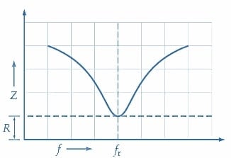
(a) Graph of impedance versus frequency

 

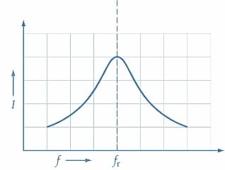
(b) Graph of current versus frequency

 

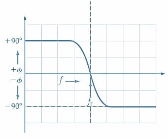
(c) Graph of current phase angle versus frequency

Figure 3. Graphs of impedance, current, and phase angle versus frequency for a series RLC circuit. Because Z=R+j(X_L-X_C), the impedance dips to R at f_r, and the current peaks. The current phase angle is zero at f_r, becomes leading below f_r and is lagging above f_r. Image used courtesy of Amna Ahmad

 

Resonance Frequency

The frequency at which resonance occurs is easily calculated by equating X_L and X_C:

\[X_{L}=2\pi f_{r}L\]

\[X_{C}=\frac{1}{2\pi f_{r}C}\]

So

\[2\pi f_{r}L=\frac{1}{2\pi f_{r}C}\]

Giving

\[f_{r}=\frac{1}{2\pi\sqrt{LC}}\,(3)\]

When L and C are in henrys and farads, respectively, Equation 2 gives f_r in hertz.

Example 1

Determine the resonance frequency for the series RLC circuit in Figure 4. Also, calculate the circuit currents at 0.25f_r, 0.5f_r, 0.8f_r, f_r, 1.25f_r, 2f_r, and 4f_r. Plot a graph of current versus frequency to a logarithmic base.

Solution

Equation 3

\[f_{r}=\frac{1}{2\pi\sqrt{LC}}=\frac{1}{2\pi\sqrt{85\mu H\times298pF}}=1MHz\]

Equation 2

\[|I|=\frac{E}{\sqrt{R^{2}+(X_{L}-X_{C})^{2}}}\]

 

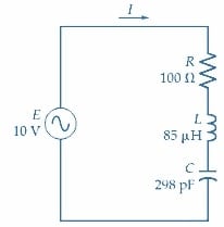
Figure 4. Circuit for Example 1. Image used courtesy of Amna Ahmad

 

The values of the various quantities are tabulated below for each frequency, and the graph of current versus frequency is plotted in Figure 5.

 

f(Hz)	XL(Ω)	XC(Ω)	(XL-XC)Ω	Z	I (mA)
250k	134	2136	-j2k	≈2k	5
500k	267	1068	-j801	≈807	12.4
800k	427	668	-j241	≈261	38.3
1M	534	534	0	100	100
1.25M	668	427	+j241	≈261	38.3
2M	1068	267	+j801	≈807	12.4
4M	2136	134	+j2k	≈2k	5

 

The graph of current versus frequency in Figure 5 clearly shows that the current rises to a maximum at the resonance frequency and falls off sharply at frequencies above and below resonance. Note from the table that when the frequency is doubled from 250 kHz to 500 kHz, the current increases from 5 mA to 12.4 mA. Also note that above resonance, the current decreases from 12.4 mA to 5 mA when the frequency is doubled from 2 MHz to 4 MHz. The same sort of corresponding current ratios is evident for other frequency changes above and below the resonance frequency. It is seen that the ratio of current to frequency is logarithmic, and so a logarithmic frequency scale is used on the graph.

 

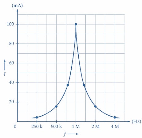
Figure 5. Plot of current versus frequency (to a logarithmic base) for a series RLC circuit. The current peaks sharply at the resonance frequency. Image used courtesy of Amna Ahmad

 

Resonance Rise in Voltage

The voltage across the resistance in a series RLC circuit is V_R=IR, and at resonance V_R equals the supply voltage [see Figure 6(a)]. As illustrated, the capacitor and inductor voltages are:

\[V_{C}=IX_{C}\,(4)\]

And

\[V_{L}=IX_{L}\,(5)\]

When the capacitor voltage levels and inductor voltage levels are calculated for various frequencies and plotted to a logarithmic frequency scale, it is found that the V_C and V_L frequency response curves are similar in shape to the circuit current-versus-frequency graph. It is also found that 

V_L and V_C at resonance can be several times greater than the supply voltage.

This effect is called the resonance rise in voltage.

Figure 6(b) shows that the waveforms of V_L and V_C are in phase opposition at resonance. Thus, the instantaneous levels of V_L and V_C cancel each other, and all the supply voltage appears across R.

 

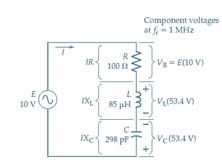
(a) Circuit and voltages at resonance

 

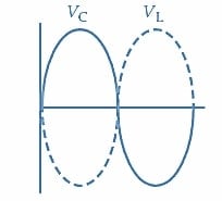
(b) Inductor and capacitor voltage waveforms

Figure 6. In a series RLC circuit, the resonance frequency V_R=E, and V_L and V_C are larger than E. V_L, and V_C are in phase opposition. Image used courtesy of Amna Ahmad

 

Example 2

For the series RLC circuit in Figure 6 (as in Example 1), determine the capacitor and inductor voltages at each frequency. Also, plot the graphs of V_R, V_C, and V_L versus frequency.

Solution

\[V_{C}=IX_{C}\,and\,V_{L}=IX_{L}\,and\,V_{R}=IR\]

The quantities are tabulated for each frequency, and the graphs are plotted in Figure 7. Note from the graph that V_C>V_L below resonance, and V_L>V_C above resonance.

 

F(Hz)	VR(V)	VL(V)	VC(V)
250k	0.5	0.67	10.7
500k	1.24	3.3	13.2
800k	3.83	16.4	25.5
1M	10	53.4	53.4
1.25M	3.83	25.5	16.4
2M	1.24	13.2	3.3
4M	0.5	10.7	0.67

 

Example 2 demonstrates that at resonance, the voltages across the capacitor and inductor become much greater than the supply voltage. The voltage across the resistance (V_R) is, of course, in phase with the circuit current, while V_L leads the current by 90° and V_C lags the current by 90°. This is illustrated in the phasor diagram in Figure 8(a). From the phasor diagram, it is clear that V_L and V_C cancel at resonance and the supply voltage is applied across the resistance.

 

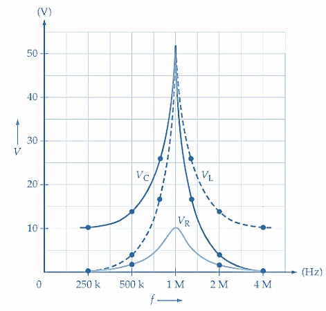
Figure 7. Graphs of capacitor voltage V_C, inductor voltage V_L, and resistor voltage V_R versus frequency (to a logarithmic base) for a series RLC circuit. At the resonance frequency, V_C and V_L become much greater than the supply voltage. Image used courtesy of Amna Ahmad

 

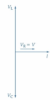
(a) Phasor diagram of a series RLC circuit at resonance.

 

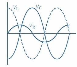
(b) Waveforms of V_L, V_C, and V_R at resonance.

Figure 8. Voltage phasor diagram and waveforms for a series RLC circuit at resonance.V_C and V_L cancel each other, V_R equals the supply voltage, and the current is in phase with the supply voltage. Image used courtesy of Amna Ahmad

 

Energy Transfer Between L and C

The waveforms of V_L, V_R, and V_C at the resonance frequency are shown in Figure 8(b). It is evident that as V_L grows positively, V_C becomes more negative, and vice versa. The positive peak of V_L occurs at the same instant as the negative peak of V_C, and the positive peak of V_C corresponds in time with the negative peak of V_L. Also, note that the positive and negative voltage peaks across the resistance coincide with the instant when V_L and V_C are zero. The information derived from these waveforms is that energy is stored in the resonant circuit. The energy is continuously transferred from the inductor to the capacitor and back again at the resonance frequency. The resonance frequency is the only frequency at which this energy transfer can take place for the particular values of the capacitor and inductor involved. Note, however, that the energy storage and energy transfer between reactive components occurs only when there is an energy input at the resonance frequency.

 

Takeaways of Determining Resonance Frequency

When a series-connected RLC circuit has the frequency of its alternating supply voltage varied, X_L = X_C at a particular frequency. The two reactances cancel, and the result is the series impedance of the circuit has a minimum value of Z=R. The circuit is in a state of resonance. The frequency at which this occurs is the resonance frequency. Because the impedance is a minimum, the series current is a maximum, and there is a rise in the voltage developed across L and C.

 

To catch up on the other articles in this series, follow these links:

• Understanding RL Circuit Operation and Time Constant
• Understanding RC Circuit Operation and Time Constant
• Examining Series RL Circuit Behavior
• Series RC Circuit Analysis

 

Featured image used courtesy of Adobe Stock