Understanding RC Circuit Operation and Time Constant

An RC circuit is a type of electrical circuit that consists of a resistor (R) and a capacitor (C) connected in series with a voltage source. The circuit operates by allowing the capacitor to charge up to the voltage of the source while the resistor limits the rate of charge. As the capacitor charges, the voltage across it increases, and the voltage across the resistor decreases. The operation of the circuit depends on the time constant (τ), which is the product of the resistance and capacitance values in the circuit.

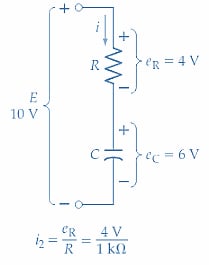
A capacitor and resistor are shown connected in series in Figure 1(a), together with a supply voltage (E) and a switch (S). The capacitor charging current flows through the resistor. So, the current can be calculated as

\[i=\frac{E_{R}}{R}\]

and

\[e_{R}=E-e_{c}\]

Giving

\[i=\frac{E-e_{C}}{R}(1)\]

If the charge on the capacitor is zero at the instant the switch is closed, then e_C = 0, and as shown in Figure 1(b)

\[i=\frac{10V-0}{1k\Omega}=10mA\]

 

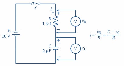
(a) Simple resistor-capacitor circuit

 

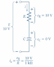
(b) Voltages at t = 0

 

(c) Voltages at t = t₁

 

(d) Voltages at t = t₂

Figure 1. The capacitor voltage in a series CR circuit tends to grow slowly from zero to its final level when the supply voltage is first switched on. Image used courtesy of EETech

 

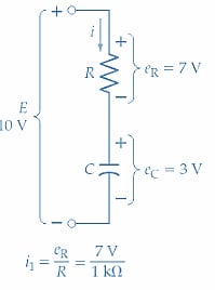
The current flow causes the capacitor to charge with the polarity illustrated. After a time t₁, the capacitor voltage might be 3 V [see Figure 1(c)]. Then the charging current becomes       

\[i=\frac{10V-3V}{1k\Omega}=7\,mA\]

It is seen that because C has accumulated some charge, the voltage across R is reduced, and consequently, the charging current is reduced from 10 mA to 7 mA. Because the charging current has been reduced, the capacitor voltage is now growing at a slower rate than before. The instantaneous levels of e_C at t = 0 and t = t₁ can now be plotted on the graph of e_C versus time; points 1 and 2 in Figure 2. 

After time t₂, the capacitor voltage has grown to 6 V [Figure 1(d)]. The charging current now becomes
\[i=\frac{10V-6V}{1k\Omega}=4\,mA\]

The charging current has been further reduced (from 7 mA to 4 mA), so the capacitor is charging at an even slower rate than before. Because the charging current has been decreasing, the time for the capacitor to charge from 3 V to 6 V is longer than the time for it to charge from 0 V to 3 V. Point 3 is plotted at t₂ and e_C = 6 V in Figure 2.

 

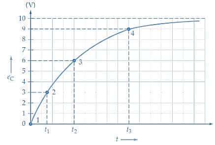
Figure 2. Graph showing the typical growth of capacitor voltage plotted versus time for a series RC circuit, starting from the instant of supply voltage switch-on. Image used courtesy of EETech

 

An even longer time is now required for the capacitor voltage to grow by another 3 V (point 4 in Figure 2). Because e_C is continuously increasing, the voltage across R is continuously decreasing, so the charging current is continuously decreasing. This means that C is charged at a rapid rate initially, then the rate decreases as the capacitor voltage grows. As in the case of the RL circuit, the terms step response and forced response are sometimes used to describe the RC circuit response to a dc input voltage.

 

Instantaneous Current and Voltage in RC Circuit

Voltage Equation

The equation for the instantaneous voltage on a capacitor in a resistive-capacitive circuit can be derived by differential calculus:

\[e_{C}=E-\Big(E-E_{o}\Big)\epsilon^{-\frac{t}{(CR)}}(2)\]

Where

e_C = capacitor voltage at time t

E = supply voltage

E_o = initial level of capacitor voltage

ε = exponential constant = 2.71

t = time, in seconds, from the commencement of the charge

C = capacitance value, in farads

R = charging resistance, in ohms

Using Equation 2, the instantaneous levels of capacitor voltage can be calculated for several different time intervals from t = 0 for a given circuit. The corresponding values of e_C and t can then be plotted to give an accurate graph of e_C versus t for the circuit. The equation can also be manipulated to obtain expressions for t, C, and R for a given capacitor voltage level. When the capacitor is initially uncharged

\[E_{o}=0\]

And

\[e_{C}=E-\Big(E\epsilon^{-\frac{t}{(CR)}}\Big)\]

Or

\[e_{C}=E\Big(1-\epsilon^{-\frac{t}{(CR)}}\Big)\]

Also, from Equation 2

\[\epsilon^{\frac{t}{(CR)}}=\frac{E-E_{o}}{E-e_{C}}\]

Taking the natural logarithm of both sides

\[\frac{t}{CR}=In\Big(\frac{E-E_{o}}{E-e_{C}}\Big)(4)\]

Equation 4 can be further simplified if the capacitor starting voltage (E_o) is assumed to be zero:

\[\frac{t}{CR}=In\Big(\frac{E}{E-e_{C}}\Big)(5)\]

Equation 5 can be used to determine t, C, or R when the other quantities are known.

Example 1

For the circuit in Figure 1(a), calculate the times t₁, t₂, and t₃ for plotting the capacitor current versus the time graph in Figure 2.

Solution

From Equation 5

\[t=CR\times ln\Big(\frac{E}{E-e_{C}}\Big)\]

At e_C = 3V

\[t_{1}=2\mu F\times1k\Omega\times ln\Big(\frac{10V}{10V-3V}\Big)\]

= 0.7ms

At e_C = 6V

\[t_{2}=2\mu F\times1k\Omega\times ln\Big(\frac{10V}{10V-6V}\Big)\]

= 1.8ms

At e_C = 9V

\[t_{3}=2\mu F\times1k\Omega\times ln\Big(\frac{10V}{10V-9V}\Big)\]

= 4.6ms

Example 2

Determine the instantaneous values of capacitor voltage at 1 ms intervals from t = 0 for the circuit in Figure 1(a).

Solution

Assuming that the initial level of capacitor voltage is zero, Equation 3 can be used.

\[e_{C}=E\Big(1-\epsilon^{-\frac{t}{(CR)}}\Big)\]

At t = 0	eC=0	point 1 in Figure 3
At t =1 ms	\[e_{C}=10V\Big(1-\epsilon^{-\frac{1ms}{2\mu F\times 1k\Omega}}\Big)=3.93\,V\]	point 2
At t = 2 ms	eC≈6.32 V	point 3
At t = 3 ms	eC≈7.77 V	point 4
At t = 4 ms	eC=8.65 V	point 5
At t = 5 ms	eC≈9.18 V	point 6
At t = 6 ms	eC≈9.5 V	point 7
At t = 7 ms	eC≈9.7 V	point 8
At t = 8 ms	eC≈9.82 V	point 9
At t = 10 ms	eC≈9.93 V	point 10
At t=∞	eC≈10 V=maximum voltage level

 

Time Constant

Referring to the graph of e_C versus t plotted in Figure 3, it is seen that when t =2 ms, e_C is 6.32 V. Note that 6.32 V is 63.2 percent of the maximum voltage level (10 V).

Also

\[t=CR=2\mu F\times 1k\Omega = 2ms\]

So, when t = CR, the instantaneous capacitor voltage level is always 63.2% of E. The quantity CR is the time constant ( ) of a resistive-capacitive circuit, and, as in the case of an RL circuit, the time constant largely determines the circuit's behavior. After a time period of 5 RC, the capacitor voltage is 99.3% of its maximum level. By drawing a straight line at a tangent to the graph of e_C / t, it can be shown that if the initial rate of charge were maintained, the capacitor voltage would reach its maximum level at a time of t =CR (see Figure 3).

 

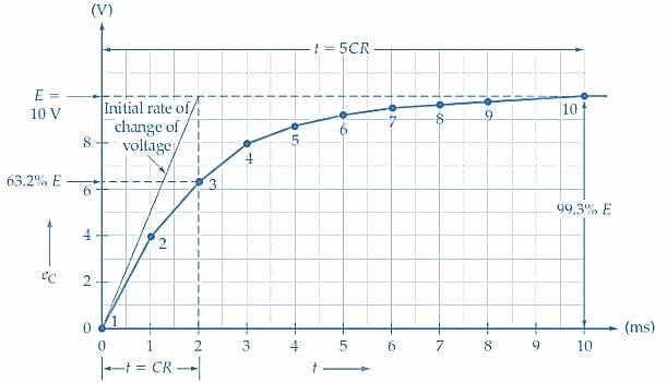
Figure 3. Graph capacitor voltage (e_C) versus time (t) for a series CR circuit. The voltage increases to 63.2% of its maximum level at t = CR and to 99.3% of its maximum at t = 5CR. Image used courtesy of EETech

 

Charging Current

Equation 3 can be manipulated to determine an equation for the instantaneous charging current at any time.

Equation 3

\[e_{C}=E\Big(1-\epsilon^{-\frac{t}{(CR)}}\Big)\]

Equation 1

\[i=\frac{E-e_{C}}{R}\]

So,
\[i=\frac{E-E{\Big(}1-\epsilon^{-\frac{t}{(CR)}}{\Big)}}{R}\]

Giving

\[i=\frac{Ee^{-\frac{t}{(CR)}}}{R}(6)\]

Alternatively, when the instantaneous capacitor voltages are known, the corresponding current levels can be determined from Equation 1.

\[i=\frac{E-e_{C}}{R}\]

The graph of i_C versus t in Figure 4 shows how the charging current changes with time. At t = 0, i_C = E/R. At t = CR, i_C has fallen by 63.2% of E/R. And at t = 5CR, i_C has fallen through 99.3% of its initial level.

 

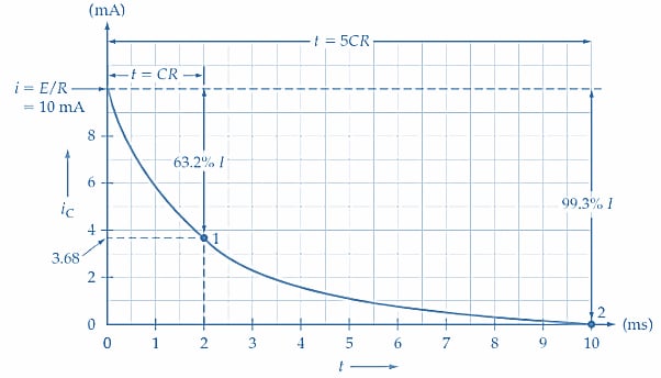
Figure 4. Graph of capacitor charging current (i_C) versus time (t) for a series CR circuit. The current falls by 63.2% of its maximum level at t = CR and by 99.3% of its maximum at t = 5CR. Image used courtesy of EETech

 

Example 3

Calculate the level of capacitor charging current for the circuit in Figure 1(a) at t =CR and t = 5CR.

Solution

At t = CR     

\[i=\frac{E\epsilon^{-\frac{t}{(CR)}}}{R}=\frac{10V\times\epsilon^{-1}}{1k\Omega}\approx3.68\,mA\,point\,1\,in\,Figure\,4\]

At t = 5 CR

\[i=\frac{10V\times\epsilon^{-5}}{1k\Omega}\approx67\mu A\,point\,2\,in\,Figure\,4\]

 

Takeaways of RC Circuit Operation

An RC circuit is an electrical circuit with a resistor and a capacitor connected in series or parallel. It is a fundamental circuit in electronics, and its behavior is governed by the interaction between the resistor and capacitor. 

In an RC circuit, the capacitor stores electrical energy in its electric field when a voltage is applied, while the resistor limits the current flow through the circuit. The behavior of an RC circuit is governed by the time constant, which is the product of the resistance and capacitance values (RC). It determines how quickly the capacitor charges or discharges in response to a voltage change.

When a voltage is applied to an RC circuit, the capacitor initially acts as an open circuit, blocking the current flow. As the capacitor charges up, it begins to conduct current, and the voltage across the capacitor decreases. Eventually, the capacitor fully charges, and the current through the circuit stops flowing.

When the voltage source is removed, the capacitor begins to discharge through the resistor. As the capacitor discharges, the voltage across the capacitor decreases, and the current through the circuit decreases. Eventually, the capacitor fully discharges, and the current through the circuit stops flowing.

The RC circuit's time constant is defined as the product of the resistance and capacitance values (RC), representing the time it takes for the capacitor to charge or discharge to 63.2% of its maximum voltage. A longer time constant means a slower charging or discharging process, while a shorter time constant means a faster charging or discharging process.

 

Featured image used courtesy of Adobe Stock