Understanding Resonance In Parallel RLC Circuits

A parallel RLC circuit contains a resistor (R), an inductor (L), and a capacitor (C) connected in parallel. Resonance in a parallel RLC circuit occurs when the reactive effects of the inductor and capacitor cancel each other out, resulting in a purely resistive circuit. The circuit exhibits interesting properties at resonance, such as a minimum current and a maximum impedance. Understanding the resonance phenomenon in a parallel RLC circuit is essential in designing and analyzing many electronic devices and systems.

 

Image used courtesy of Adobe Stock

 

Ideal Parallel Resonant Circuit

Consider the parallel RLC circuit in Figure 1(a). The admittance of the circuit is:

\[Y=\frac{1}{R}-j\frac{1}{X_{L}}+j\frac{1}{X_{C}}\]

If the supply frequency is adjusted until X_L and X_C are equal, the admittance is:

\[Y=\frac{1}{R}\]

 

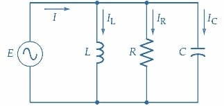
(a) Parallel RLC circuit with a variable frequency source

 

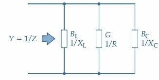
(b) B_L and B_C vary with the frequency of the source.

Figure 1. Ideal parallel resonance circuit. At resonance, X_L=X_C, I=E/R, and I_C and I_L are much larger than I. Image used courtesy of Amna Ahmad

The circuit impedance is:

\[Z=R\]

Consequently, the current taken from the supply source is:

\[I=\frac{E}{R}\]

And the currents through the inductor and capacitor are:

\[I_{L}=\frac{E}{X_{L}}\,\,\,and\,\,\,I_{C}=\frac{E}{X_{C}}\]

I_L and I_C are normally much larger than the supply current at resonance. The resistor current (in the circuit in Figure 1) is in phase with the supply voltage, the inductor current lags the supply voltage by 90°, and the capacitor current leads the supply voltage by 90°. This is illustrated by the phasor diagram in Figure 2(a) and by the current waveforms in Figure 2(b). When X_L and X_C are equal, the inductive and capacitive currents are equal and opposite, as illustrated in the phasor diagram. Thus, the total current supplied by the voltage source is IR. Currents I_C and I_L result from the energy stored in the circuit being continuously transferred from the inductor to the capacitor and back again.

 

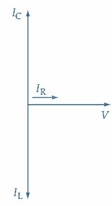
(a) Phasor diagram for a parallel resonance circuit

 

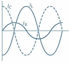
(b) Waveforms of I_C, I_L, and I_R at resonance

 Figure 2. Current phasor diagram and waveforms for an ideal parallel resonance circuit. I_C and I_L cancel each other, and the total supply current is I_R, which is in phase with the supply voltage. Image used courtesy of Amna Ahmad

 

Practical Parallel Resonant Circuit

A practical inductor is not purely reactive but has a winding resistance, and this must be represented as a resistance R_W in series with an inductance L. Some capacitors must also be shown as having a resistive component; however, capacitors generally can be assumed to be purely reactive. The circuit in Figure 3(a) is a practical parallel LC circuit, and the phasor diagram in Figure 3(b) represents the circuit conditions at resonance. It is seen that the presence of the resistive component in the inductive branch makes the I_L phase angle (ɸ) slightly less than 90°. Resonance is achieved when the vertical component of I_L [I’_L in Figure 3(b)] is equal to the capacitor current (I_C).

 

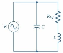
(a) Parallel LC circuit

 

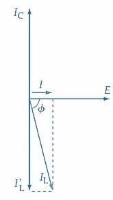
(b) Phasor diagram for a practical parallel LC circuit

Figure 3. In a practical parallel resonance circuit, the presence of a resistive component in the inductance gives an inductor current phase angle less than 90° at resonance. Image used courtesy of Amna Ahmad

 

The admittance of the parallel circuit in Figure 3(a) is:

\[Y=\frac{1}{R_{W}+jX_{L}}+j\frac{1}{X_{C}}\]

Multiplying

\[\frac{1}{R_{W}+jX_{L}}\,\,\,by\,\,\,\frac{R_{W}-jX_{L}}{R_{W}-jX_{L}}\]

results in:

\[Y=\frac{R_{W}}{R^{2}_{W}+X^{2}_{L}}-j\frac{X_{L}}{R^{2}_{W}+X^{2}_{L}}+j\frac{1}{X_{C}}(1)\]

For the circuit to become purely resistive at resonance

\[\frac{1}{X_{C}}=\frac{X_{L}}{R^{2}_{W}+X^{2}_{L}}\]

Or

\[{X_{C}}=\frac{R^{2}_{W}+X^{2}_{L}}{X_{L}}(2)\]

and Equation 1 gives the admittance at resonance as

\[Y=\frac{R_{W}}{R^{2}_{W}+X^{2}_{L}}\]

So, the circuit impedance at resonance is

\[Z=\frac{R^{2}_{W}+X^{2}_{L}}{R_{W}}\]

From Equation 2

\[X_{L}X_{C}=R^{2}_{W}+X^{2}_{W}\]

Therefore,

\[Z=\frac{X_{L}X_{C}}{R_{W}}=\frac{2\pi f_{r}L}{2\pi f_{r}CR_{W}}\]

So, at resonance

\[Z=\frac{L}{CR_{W}}(3)\]

and this is a resistive quantity.

When the impedance of the parallel LC circuit (as represented by the inverse of Equation 1) is plotted to a logarithmic frequency base, the impedance peaks at the resonance frequency, as shown in Figure 4(a). Therefore, a parallel LC circuit has a maximum impedance at the resonance frequency.

The series resonant circuit has a minimum impedance at the resonance frequency. So, the impedances of series and parallel LC circuits at resonance are opposites. As a consequence of the peak in the impedance value of a parallel resonant circuit, there is a dip in the current taken from the supply at the resonance frequency. This is illustrated in Figure 4(b). Once again, this is the opposite of the case with series resonance.

 

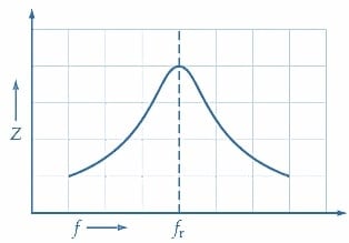
(a) Impedance versus frequency

 

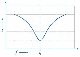
(b) Current versus frequency

Figure 4. Graphs of impedance and current versus frequency for a parallel RLC circuit. Because X_L and X_C cancel each other at f_r, the impedance peaks to Z=L (CR_W), and the current dips. Image used courtesy of Amna Ahmad

 

Phase Angle

The impedance of a parallel LC circuit is resistive at the resonance frequency. At supply frequencies below resonance, the inductive reactance is smaller than the capacitive reactance, as shown in Figure 5(a).

 [(2πfL)] <1/(2πfC)]

Thus, the inductive current is greater than the capacitive current, and the total supply current lags the supply voltage. This effect becomes most pronounced at frequencies well below f_r so that, as shown in Figure 5(c), the current phase angle is close to -90°.

When the supply frequency is above f_r, the capacitive reactance becomes smaller than the inductive reactance, as shown in Figure 5(b).

[1/(2πfC) <(2πfL)]

In this case, the capacitor current is larger than the inductor current, and the total supply current leads to the supply voltage. As illustrated in Figure 5(c), the current phase angle is close to 90° at frequencies well above resonance.

 

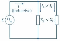
(a) When fr, X_LC, and I are largely inductive

 

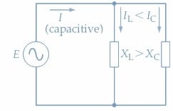
(b) When f>f_r, X_L>X_C, and I are largely capacitive

 

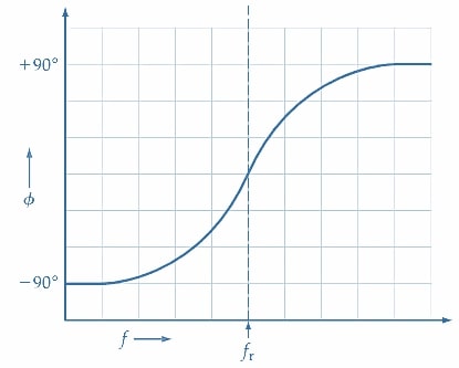
(c) The current phase angle lags at frequencies below f_r and leads at frequencies above f_r.

Figure 5. A parallel resonant circuit has a 90°phase angle at supply frequencies well below resonance. This changes to zero as the resonance frequency is approached and then approaches 90° at frequencies well above resonance. Image used courtesy of Amna Ahmad

 

Example 1

A parallel LC circuit, as in Figure 3(a), has E=100 mV, L=150 µH, R_W=15 Ω, and C =750 pF. Calculate the supply current at resonance.

Solution

Equation 3

\[Z=\frac{L}{CR_{W}}=\frac{150\mu H}{750pF\times 15\Omega}=13.3k\Omega\]

\[I=\frac{E}{Z}=\frac{100mV}{13.3k\Omega}=7.52\mu A\]

 

Takeaways of Resonance In Parallel RLC Circuits

When a parallel-connected RLC circuit has the frequency of its alternating supply voltage varied, it is found that X_L = X_C at a particular frequency. The two reactances cancel. The result is the circuit impedance has a maximum value, and the circuit current is a minimum, but there is a rise in the L and C current levels. An RLC circuit can be tuned to resonate over a range of frequencies by making L or C adjustable.