Inductors in Series

For inductors connected in series with no mutual flux coupling, the electrical effect is analogous to resistors connected in series and the individual inductance values are simply added together.

 

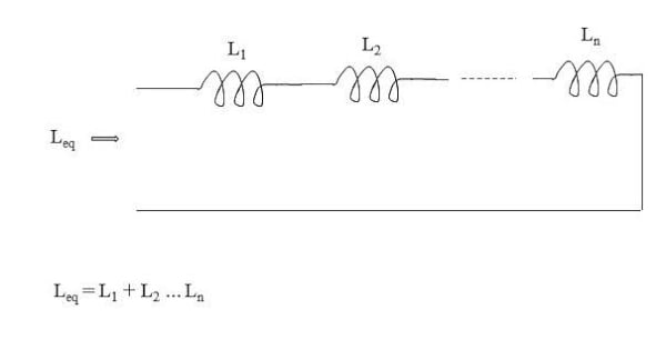
Figure 1. The equivalent inductance of series-connected inductors. Image used courtesy of Blaine Geddes

 

Derivation

The equivalent inductance looking into series connected inductances is easily derived from first principles (basic electric circuit theory) as shown in Figure 2. The inductor is characterized by having a voltage developed across it that is the product of its self-inductance and the rate of change of current flowing through it. Since a common current flows through all elements of this series circuit, the rate of change of current is the same for all the series elements. The common di/dt term cancels, resulting in the equivalent inductance being the sum of the individual inductances.

 

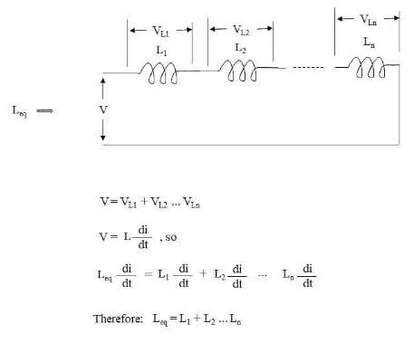
Figure 2. Derivation of the equivalent inductance of inductors connected in series. Image used courtesy of Blaine Geddes

 

The Time Constant of an L-R Circuit

In this EE Power article, the basic example circuit of Figure 3 was presented for which a solution to the differential equation was found to be: 

\(i=\frac{V}{R}-\frac{V}{R}e^{-\frac{Rt}{L}}\)

[1]

At time t=0, the switch closes, but i = 0, because the inductor looks like an infinite impedance in response to an idealized instantaneous increase in current flow. Current ramps according to the exponential function to reach a steady state at a value of V/R for the DC circuit because an ideal inductor has no impedance at zero frequency. The differential equation of Equation [1] satisfies those boundary conditions.

A common parameter for characterizing a basic R-L or R-C circuit is its time constant, which is defined as the time for some quantity to reach a value within 1/e of its final value, or about 63% of the final value. For equation [1], the exponential rise in current is shown in Figure 4, and the time constant is L/R.

 

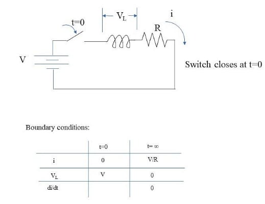
Figure 3. DC transient analysis of an inductor with a series resistor. Image used courtesy of Blaine Geddes

 

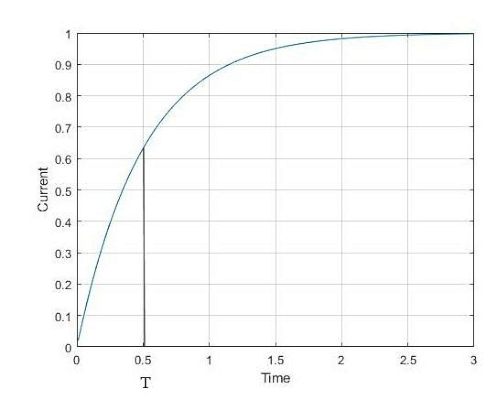
Figure 4. Equation 1 plotted for V=2, R=2, L=1. The time constant is L/R = 0.5. Image used courtesy of Blaine Geddes

 

Applications of Series Inductors

A series inductor is most often used to limit surge currents, such as the surge current of a motor starting,  to suppress high-frequency signals, for example, to suppress high frequency switching signals from leaking onto a power rail, or as a choke to limit ripple from a DC power supply derived from rectified AC. Inductors are also used in tuned circuits, lumped element filter design, and impedance matching to cancel capacitive reactance at a discrete frequency.

The inductor is an effective current surge suppressor because it develops a voltage across it that is proportional to the rate of change of current flow through it. Therefore, an instantaneous change in current is opposed by a back emf that tends to infinity. The idealized model of an inductor is that it represents an open circuit to an instantaneous change in current. In the real world, nothing happens in a time interval of zero, so even an ideal inductor can not generate an infinite voltage in a real circuit, but it can generate a very high voltage if a large steady state current through an inductor is suddenly interrupted. 

 

Filters

Inductors and capacitors can be combined to form a basic filter. Filters are important throughout electrical engineering and are heavily used in communications circuits, especially radio. Although the significance of the analog lumped element filter is diminishing as communications electronics increasingly shift to the digital domain, the analog filter is still important. Filters are also used in audio circuits, control systems, and power supplies for filtering ripple and harmonics.

A simple two-element low pass filter and the derivation of its transfer function are shown in Figure 5. Interchanging the positions of the inductors and capacitors would produce a high-pass response.

 

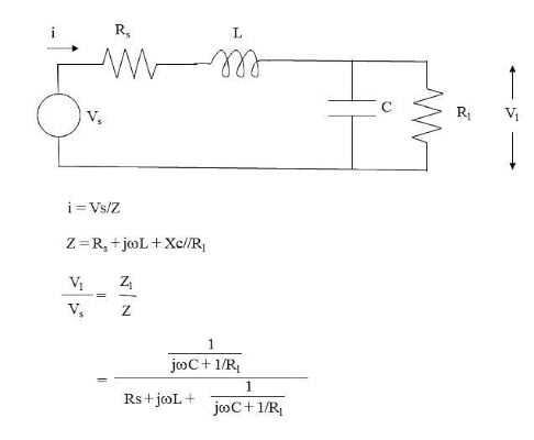
Figure 5. A two-element LC low-pass filter and its transfer function. Image used courtesy of Blaine Geddes

 

Plotting the voltage transfer function of Figure 5 versus frequency yields the representative plot of Figure 6, where R, L, and C are all set to 1. The code generating the plot is shown below:

C=1;

Rl=1;

Rs=1;

L=1;

j=sqrt(-1);

f=0.01:0.01:1;

 

Zl = 1./(j.*2.*pi.*f.*C + 1./Rl);

Z = Rs + j.*2.*pi.*f.*L + Zl;

vl_vs = 20.*log10(abs(Zl./Z))+6;

 

plot(f,vl_vs);

grid

 

xlabel('Frequency (Hz)')

ylabel('Magnitude Response(dB)')

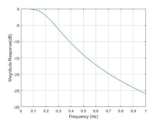
Figure 6. Magnitude response of the transfer function for the two-element low pass filter of Figure 5. Image used courtesy of Blaine Geddes

 

The concept of the basic two-element low-pass LC filter with series inductors and shunt capacitors can be extended to the standard ladder structure of Figure 7. 

 

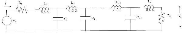
Figure 7. Low-Pass LC ladder network. Image used courtesy of Blaine Geddes

 

Analyzing the lumped element ladder network is straightforward in principle, but the algebra rapidly gets unwieldy for more than a few elements. Manual calculation would become impractical beyond a few elements, but the basic algebra is computationally simple and easily programmed. The basic MATLAB code shown above could be extended easily enough to plot the response of a larger ladder structure. Mathematical software such as MATLAB can handle complex numbers with polar to rectangular conversions done implicitly which simplifies the code. Synthesizing a ladder structure to produce a certain response is much more mathematically involved and well beyond the scope of this article, but filters are so fundamental to electrical engineering that the subject has been well studied with entire texts written on the subject. 

For the ladder structure of Figure 7, two standard filter types are commonly implemented. These are known as Butterworth and Chebyshev (or Tchebyscheff) filters. The Butterworth filter response is characterized by a mostly flat passband response, but with some attenuation towards the upper limit of the passband. The Chebyschev filter is characterized by steeper roll-off than the Butterworth filter, but at the price of ripple in the passband with a ripple magnitude that depends on the component values selected. Both filter types offer monotonically increasing attenuation as frequency increases. 

Filter tables are available for filter design where normalized component values are tabulated for a given filter order and choice of maximum passband attenuation. The maximum attenuation in the passband is at the upper passband edge for the Butterworth filter and appears as ripple throughout the passband for the Chebyshev filter. Such a set of tables are published in reference 1. The component values are normalized to some source resistance and cutoff frequency. For the tables of reference 1, this is 1 Hz and 1 ohm. Component values for any other cutoff frequency (F_ref) and source resistance (R_ref) are obtained by scaling, where:

L_ref = R_ref/2πF_ref

Cref = 1/(2πF_ref R_ref)

Each of the tabulated component values is then multiplied by L_ref or C_ref to obtain the respective actual L and C values. 

Tabulated values for a low-pass filter can be used for an equivalent high-pass filter with the inverse frequency response by swapping the inductors and capacitors in the ladder structure. 

A third standard filter response is that of the elliptic filter. Unlike the monotonically increasing attenuation behavior with increasing frequency of both the Chebyshev and Butterworth low pass filters, the elliptic filter is characterized by a stopband attenuation floor with ripple throughout both the passband and stopband. The advantage of the elliptic filter is that it offers the steepest roll-off for a given filter order. The price is a more complicated filter structure where the basic low pass ladder of Figure 7 is modified to that of Figure 8 or Figure 9. As with the Chebyshev and Butterworth filters, converting the reference low pass elliptic filter to a high pass equivalent requires interchanging the L and C components.

 

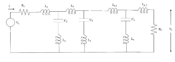
Figure 8. Low pass lumped element filter structure for implementing an elliptic response. Image used courtesy of Blaine Geddes

 

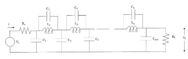
Figure 9. Alternative low pass lumped element filter structure for implementing an elliptic response. Image used courtesy of Blaine Geddes

For any filter design, a component sensitivity analysis is an important exercise to ensure the filter response is not overly affected by component tolerances. At high frequencies, component parasitic effects and track lengths become significant. As noted in this EE Power article, a chip inductor becomes a capacitor at some frequency.

 

Featured image used courtesy of Adobe Stock