Understanding RL Circuit Operation and Time Constant

An RL circuit is a type of electrical circuit that includes a resistor and an inductor connected in series. When a voltage is applied to the circuit, an electric current flows through the resistor and the inductor. The inductor resists changes in the current flow by creating a magnetic field around it, which induces a voltage across the inductor that opposes the current flow. This property of the inductor is what gives an RL circuit its characteristic behavior, including transient response and a time constant.

When switch S₁ is closed in the simple battery and resistor circuit shown in Figure 1(a), the current jumps instantaneously to its maximum level of I=E/R. This is illustrated by the graph of i versus t in Figure 1(b), and it assumes that R is purely resistive.

 

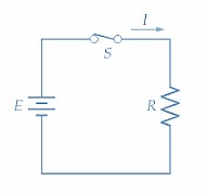
(a) Simple resistance circuit

 

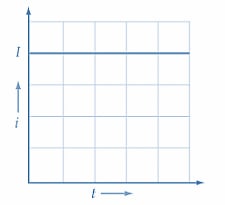
(b) Graph of current versus time for a simple resistance circuit

Figure 1. In a simple resistance circuit, the current tends to jump to its final level and remain constant. Image used courtesy of EETech

 

Now consider the circuit shown in Figure 2(a) and assume that L is a pure inductance. When the current changes through an inductor, a counter-emf is generated with the value

\[e_{L}=L\frac{\Delta i}{\Delta t}\,volts\]

The counter-emf opposes the current change that generates it, so, as shown in the circuit, its polarity is such that it opposes the current (i). Using Kirchhoff’s voltage law, the instantaneous current level is

\[i=\frac{E-e_{L}}{R}(1)\]

Although the actual current level is very small when S is first closed, its rate of growth is large. The initial rapid rate of current growth causes the counter-emf (e_L) to be virtually equal to the supply voltage (E). This is illustrated in Figure 2(b). Putting e_L = E into Equation 1 and using the voltage and component values shown in the circuit, the initial current level is

\[i_{o}=\frac{10V-10V}{1k\Omega}=0\]

 

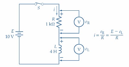
(a) Simple resistor-inductor circuit

 

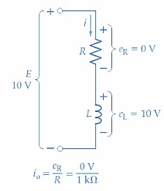
(b) Voltages at t = 0

 

(c) Voltages at t = t₁

 

(d) Voltages at t = t₂

Figure 2. The counter-emf generated in an inductor when the current level changes causes the current in an RL circuit to grow slowly to its final level when the supply voltage is switched on. Image used courtesy of EETech

 

So, on the graph of i versus t, i is zero at t = 0; point 1 in Figure 3. At this instant, the rate of change of current \((\frac{\Delta i_{o}}{\Delta t_{o}}\,on\,the\,graph)\) is at its maximum value. Because \(e_{L}=L\frac{\Delta i_{o}}{\Delta t_{o}},\,e_{L}\) also has its maximum level at t = 0.

 

Figure 3. Graph showing the typical growth of current plotted versus time for a series RL circuit, starting from the instant of supply voltage switch-on. Image used courtesy of EETech

 

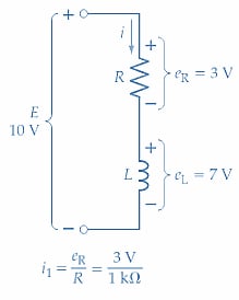
Some time t₁ after S is closed, the rate of change of current has decreased to a value (∆i1∆t1 on the graph in Figure 3) that gives e_L=7 V. So, from Figure 2(c), at time t₁ the instantaneous current level is

\[i_{o}=\frac{10V-7V}{1k\Omega}=3mA\]

Current i₁=3 mA is plotted at time t₁ on the graph of i versus t; point 2 in Figure 3.

Because e_L is falling, the current level is increasing. As the current level grows, it gets closer to its maximum level of I=E/R, and in doing so, the rate of change of current ∆i/∆t continues to decrease. This decrease in ∆i/∆t is the cause of the decreasing level of counter-emf (e_L=L∆i/∆t).

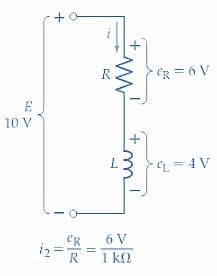
After some time t₂, ∆i/∆t has fallen to a level that gives e_L = 4 V. So, from Figure 2(d)

\[i_{o}=\frac{10V-4V}{1k\Omega}=6mA\]

Current i₂ = 6 mA is plotted at time t₂ in Figure 3; point 3. At time t₃, ∆i/∆t is such that e_L = 1 V, giving

\[i_{o}=\frac{10V-1V}{1k\Omega}=9mA\]

The value of i₃ is plotted on the graph at time t₃, point 4. The final current level when e_L becomes zero is, of course, I=E/R.

Because the counter-emf is initially large and falls off smoothly to zero, the current grows continuously from zero to its maximum level, as illustrated in Figure 3. As the current approaches maximum, the rate of change of current (∆i/∆t) keeps decreasing, and this produces the decreasing level of e_L. The terms step response and forced response are sometimes used to describe the RL circuit response to a DC input voltage.

 

Instantaneous Current and Voltage in an RL Circuit

Current Equation 

By application of calculus, it can be shown that the equation for instantaneous current in an inductive-resistive circuit is

\[i=\frac{E}{R}\Big(1-\epsilon^{-\frac{tR}{L}}\Big)(2)\]

Where

i = instantaneous current, in amperes, at time t

E = supply voltage

R = series resistance, in ohms (including the winding resistance of the inductor)

ε = exponential constant =2.718

t = time, in seconds, from the current commencement 

L = inductance of the inductor, in Henry

Using Equation 2, the instantaneous current levels can be calculated for several different time intervals from t = 0 for a given circuit. The corresponding values obtained in this way can be used to plot an accurate graph of i versus t for the circuit. Equation 2 can also be manipulated to determine the value of t, R, or L for a given current level.

\[\epsilon^{-\frac{tR}{L}}=\frac{E}{E-iR}\]

Taking the natural logarithm of both sides

\[t\frac{R}{L}=In\,ln\Big(\frac{E}{E-iR}\Big)(3)\]

Example 1

For the circuit in Figure 2(a) calculate the times t₁, t₂, and t₃ for plotting the inductor current versus the time graph in Figure 3.

Solution

From Equation 3

\[t=\frac{L}{R}In\,ln\Big(\frac{E}{E-iR}\Big)\]

At i = 3 mA

\[t_{1}=\frac{4H}{1k\Omega}Inln\Big(\frac{10V}{10V-(3mA\times1k\Omega)}\Big)=1.45\,ms\]

At i = 6 mA

\[t_{1}=\frac{4H}{1k\Omega}Inln\Big(\frac{10V}{10V-(6mA\times1k\Omega)}\Big)=3.7\,ms \]

At i = 9 mA

\[t_{1}=\frac{4H}{1k\Omega}Inln\Big(\frac{10V}{10V-(9mA\times1k\Omega)}\Big)=9.2\,ms\]

Example 2

Determine the instantaneous levels of current at 2 ms intervals from t =0 for the circuit of Figure 2(a).

Solution

Equation 2

\[i=\frac{E}{R}\Big(1-\epsilon^{-\frac{tR}{L}}\Big)\]

At t = 2 ms	\[i=\frac{10V}{1k\Omega}\Big(1-\epsilon^{\frac{-2ms\times1k\Omega}{4H}}\Big)\approx3.94\,mA\]	Point 2
At t = 4 ms	\[i=\frac{10V}{1k\Omega}\Big(1-\epsilon^{\frac{-4ms\times1k\Omega}{4H}}\Big)\approx6.32\,mA\]	Point 3
At t = 6 ms	i=7.77 mA	Point 4
At t = 8 ms	i=8.65 mA	Point 5
At t = 10 ms	i=9.18 mA	Point 6
At t = 12 ms	i=9.5 mA	Point 7
At t = 14 ms	i=9.7 mA	Point 8
At t = 16 ms	i=9.82 mA	Point 9
At t = ∝	i=10 mA=maximum current level

 

The corresponding values of t and i are plotted in Figure 4.

Time Constant

Referring to the graph of i versus t plotted in Figure 4, it is seen that when t = 4 ms, i is 6.32 mA. Note that 6.32 mA is 63.2% of the maximum current level (10 mA). Also

\[\frac{L}{R}=\frac{4H}{1k\Omega}=4\,ms=t\]

So, when t =L/R, the instantaneous current level is always 63.2% of E/R. The quantity L/R is termed the time constant of an inductive-resistive circuit, and the time constant is very important in determining the behavior of the circuit. Sometimes the Greek letter is used as the symbol for the time constant. It can be shown that after a time of t = 5L/R, the current is 99.3% of its maximum level (see Figure 4). By drawing a straight line from the origin at a tangent to the graph of i versus t, it is seen that if the initial rate of change of current were maintained, the current would reach its maximum level at a time of t = L/R.

 

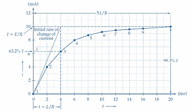
Figure 4. Graph of current(i) versus time (t) for a series RL circuit, as determined in Example 2. The current increases to 63.2% of its maximum level at t = L/R and to 99.3% of its maximum at t = 5L/R. Image used courtesy of EETech

 

Counter-emf

Equation 2 can be manipulated to derive an equation for the instantaneous counter-emf at any time.

Equation 2

\[i=\frac{E}{R}\Big(1-\epsilon^{-\frac{tR}{L}}\Big)\]

So

\[iR=E=E\epsilon^{-\frac{tR}{L}}\]

From Equation 1

\[iR=E-e_{L}\]

So

\[E-e_{L}=E-E\epsilon^{-\frac{tR}{L}}\]

Giving

\[e_{L}=E\epsilon^{-\frac{tR}{L}}(4)\]

Alternatively, when the instantaneous current levels have been calculated, the corresponding emf values can be determined from Equation 1.

\[e_{L}=E-iR\]

Example 3

Calculate the level of the counter-emf for the circuit in Figure 2(a) at t = L/R and t = 5L/R.

Solution

At t = L/R

Equation 4

\[e_{L}=E\epsilon^{-\frac{tR}{L}}=10\epsilon^{-1}\approx3.68\,V(Point\,1\,in\,Figure\,5)\]

At t = 5L/R

\[e_{L}=E\epsilon^{-\frac{tR}{L}}=10\epsilon^{-5}\approx0.067\,V(Point\,2\,in\,Figure\,5)\]

The graph of e_L versus t in Figure 5 shows how the counter-emf (e_L) changes with time. At t =0, e_L equals the supply voltage (E). At t = L/R, e_L has fallen by 63.2% of E, and at t = 5L/R, e_L has fallen through 99.3% of its initial level. Comparing the graphs of i versus t and e_L versus t, it is seen that the inductor terminal voltage drops as the current increases.

 

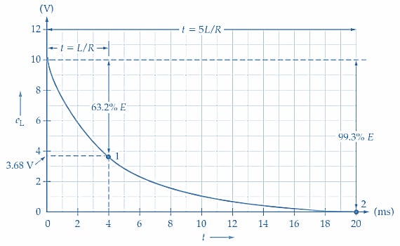
Figure 5. Graph of inductor voltage (e_L) versus time (t) for a series RL circuit. The voltage falls by 63.2% of its maximum level at t = L/R and by 99.3% of its maximum at t = 5L/R. Image used courtesy of EETech

 

Takeaways of RL Circuit Operation

An RL circuit is an electrical circuit consisting of a resistor (R) and an inductor (L) connected in series. When an electric current flows through the circuit, it creates a magnetic field around the inductor. This magnetic field induces a voltage across the inductor that opposes the current flow.

The behavior of an RL circuit can be described using the following equations:

• The voltage across the resistor (e_R) is equal to the current (i) multiplied by the resistance (R): e_R=iR.
• The voltage across the inductor (e_L) is equal to the inductance (L) multiplied by the rate of change of the current: \(e_{L}=L\frac{\Delta i}{\Delta t}\).
• The total voltage (E) applied to the circuit is equal to the sum of the voltage across the resistor and the voltage across the inductor: \(E=e_{L}+e_{R}\)

Using these equations, one can derive the differential equation that describes the behavior of an RL circuit over time.

\[L\frac{\Delta i}{\Delta t}+iR=E\]

Solving this equation yields the current as a function of time, which can be used to analyze the behavior of the circuit.

The time constant of an RL circuit is given by L/R, which determines how quickly the circuit reaches its steady state. A larger inductance or resistance will result in a longer time constant and slower response.

 

Featured image used courtesy of Adobe Stock