Facebook
 Google
 GitHub
 Linkedin
Temperature Limits for Power Modules – Part 2: Lifetime
This article talks about calculating if the module internal interconnects could withstand the temperature swings and meet the design lifetime specification.
In part 1 the limit of maximum junction temperature was discussed. Here in part 2, a second thermal limit, due to wear out caused by temperature cycling will be illustrated using an example from a real-life application.
Introduction
The effects of wear out in power modules due to temperature cycling should be carefully considered in any power electronics design, especially in applications with high cyclical loading and long life requirements. Semiconductor packages are constructed using different materials, which have different rates of thermal expansion, expressed as coefficients of thermal expansion, CTE. Temperature cycles induce stress in the dissimilar materials, eventually causing degradation of the joints between these materials. In a typical power module with baseplate this degradation occurs in three places: at the chip level, on the top side where the bond wires attach to the top metallization surface of the chip; on the bottom side where the chip is soldered to the Direct Copper Bonded (DCB) ceramic and in the system solder joint between the DCB ceramic and the baseplate. Long term temperature cycling testing at the chip level is achieved through active power cycling tests where a typical temperature cycle lasts several seconds, referred to as Power Cycling seconds (PCsec) testing. For the system solder the test temperature cycle lasts several minutes and is referred to as Power Cycling minutes (PCmin) testing.

Figure 1: Four corners of center DCB used for temperature variation simulations.
Converter Design Requirements
The application example shown here is for a three-phase grid-tie converter. The lifetime specification for the converter was to meet a 12-year life operating 24/7. The design was based on a 300A 1200V EconoDUAL™ 3 module from Infineon Technologies mounted on an air-cooled heat sink. The end-user provided a mission profile of the application by measuring the load over a typical 5 day time period sampled at 1-second intervals.
Methodology
The estimation of lifetime was sub-divided into the following five steps.
- Mission profile. This describes the actual operating conditions in the end application over a typical time period. This can be the hardest part of any calculation as real data is often not available. If no real data is available, it is recommended to perform analysis with a best estimate of the mission profile.
- Loss calculation. Calculate the semiconductor losses as they change over the time period of the mission profile. A simple calculation can often be used to decide if PCsec or PCmin is the limiting life factor for a given profile to reduce the number of required calculations.
- Temperature variation. Using a thermal model of the module, the temperature changes of the chips and the system solder layer during the mission profile can be calculated. If PCsec is the limiting factor, the temperature changes of both IGBT and Diode chips should be calculated.
- Rain flow quantization. Using a rain flow method algorithm the delta T excursions can be extracted from the temperature profile and then quantized or binned into their different delta T ranges. For example all the delta T excursions between 27.5°C and 32.5°C can be grouped together in the same bin with a delta T of 30°C
- Lifetime estimation from supplier data. The % of lifetime consumed for each bin of delta T events can be estimated using graphs showing the statistical degradation at specific delta T levels provided by the module supplier. The % lifetime of all the bins can then be summed to provide total percentage of the design life used over the complete mission profile. Note this does assume that all degradation will sum linearly.
Worked Example
Mission Profile and Loss Calculator
With the end-user providing more than 400,000 data points for the load mission profile the first step was to somehow reduce the number of data points for analysis; but how does one decide which time periods are typical or worst case? To assist with the initial evaluation the data was divided up into 135 blocks consisting of 3200 samples each (approx. 53 minutes’ worth of data). The load values of each block were integrated and the blocks with the highest levels plotted. One block was selected for analysis, which, using engineering judgement, had significant load peaks and troughs which produce large delta T’s. Using the Infineon on-line tool, Iposim, the losses at several load points were calculated for both the IGBT and the diode chips. A curve fit was applied to these losses vs. load points to enable a simple interpolation of losses at any load point. Note the task here was simplified as both the fundamental frequency (of the grid) and switching frequency of the IGBT’s are fixed. When more variables are involved this loss estimation becomes more complex. After performing an initial estimate calculation on the changes in temperature it was clear that the PCmin would be the limiting factor as at a grid fundamental frequency there is a low-temperature ripple on the chips.
Temperature Variation and Rain Flow Quantization
The next step in the calculation was to estimate the change in temperature of the solder layer between the DCB and the baseplate over the loss profile, as any degradation of this solder layer, and it’s resultant increase in chip thermal resistance is dependent primarily on changes in temperature, delta T. Using a validated Finite Element Model (FEA) of the module the temperature of the system solder layer at the corners of the DCB could be simulated see Figure1. The corners are used as this is where the stress is the highest and where the degradation or delamination starts (1).

Figure 2: Temperature variation in DCB temperatures with a 5-second power pulse.
Figure 2 shows the temperature variation during a 10-second load cycle. Running a full FEA model for a 53-minute transient loss profile is not practical. A much simpler method is to use the FEA model to derive an electrical equivalent circuit Foster model that describes the transient thermal characteristics of the solder layer with respect to dynamic power loss. The model can be derived by applying a constant power, in the FEA model, to both the IGBT and diode chips. Once the steady-state temperature was reached, the power was removed, and the cooling curve of the average temperature of the corners of the system solder layer was recorded, see Figure 3.

Figure 3: Cooling curve of corners of the DCB derived from the FEA model.
From this cooling curve, a third-order Foster model was derived as shown in Figure 3. The block of 3200 power loss values from step 1 were then fed into the 3rd order Foster model and delta T values obtained as shown in Figure 4.

Figure 4: Center DCB power loss in Watts and calculated Avg. DCB corner temperature vs. time.
From this temperature profile, the delta T values were extracted and binned using a rain flow algorithm. In this application, the ambient temperature changes could be ignored as the converter was operating in a climate-controlled environment, however, ambient changes typically need to be considered in the mission profile.
Lifetime estimation
The % of design lifetime used by each bin could then be calculated using data provided by Infineon. This data, provided in graphical form, shows how many cycles it will take at any given delta T for the module to reach the end of its defined design life, (the definition of life being a 20% increase in thermal resistance junction to case). For example, from the rain flow analysis of the data shown in Fig 4 there is a single delta T event in the Δ30°C bin. For a 12 year life, that equates to ≈120,000 temperature cycles at a delta of 30°C. The defined design life for a delta T of 30°C is ≈ 500,000 cycles, so ≈24% of the lifetime is used by this bin. Summing all the bins the estimated percentage of total life used in 12 years is 54%. Expressed another way the end of design life is estimated to be 22 years.
The Next Level
In this estimation, engineering judgement was used together with assumptions and omissions to reduce the work and arrive at 90% of the answer with 10% of the work. The calculations shown here, took 1-2 days of work once the FEA model was available. Note a close collaboration with the module vendor is strongly recommended to fully understand the correlation between the actual mission cycle and the supplier test data provided (2), also to assess the possible effect of any assumptions made in the calculation. Some possible options that could be considered to help provide a more accurate result:
- Running a full rain flow on all 135 data blocks and considering design life for min, max and average time blocks.
- Including changes in ambient temperature and changes in lifetime due to the temperature cycle starting temperature.
- Considering the increase in thermal resistance due to delamination of solder layers and degradation of any Thermal Interface Material (TIM).
- Calculating the variation in the Foster model with different IGBT chip loss to Diode loss ratios.
If these and other second-order effects are taken into account and failure modes of other components such as capacitors and fans are included then any lifetime reliability estimations of the converter can be very time-consuming. It should be remembered that all these calculations are based on a statistical analysis and are only as good as the input data. So how much is enough? Some questions that might help frame the answer to that difficult question are: what is the cost of a converter failure, how often do the worst-case conditions really occur, how accurate is the mission profile and base loss and temperature calculations, what is the actual realistic lifetime requirement and finally, as a design engineer, how well do you want to sleep at night? It is also possible to implement in the system controls an on-line lifetime estimator, and so be able to act preemptively with preventive maintenance if the customer has subjected the converter to an especially severe mission profile.
Conclusion
In these two articles, we have considered two different corner points in the thermal design of IGBT based power modules. In part 1, the focus was keeping the semiconductor itself below the maximum operating temperature; in part 2, the focus was on calculating if the module internal interconnects could withstand the temperature swings and meet the design lifetime specification of the product. These two corner points can be mutually exclusive and it is recommended that both these thermal constraints be considered as key components of any design review process.
About the Authors
Jeremy Howes worked as a principal engineer at Parker Hannifin that is an engineering company with expertise that spans the core motion and control technologies – Climate Control, Electromechanical, Filtration, Fluid & Gas Handling, Hydraulics, Pneumatics, Process Control and Sealing & Shielding.
Greg Shendel has a BSE & BSA degree in the Field of Mechanical/Manufacturing Engineering & Engineering Management at Miami University. He worked as a Mechanical Engineer III at Parker Hannifin that is an engineering company with expertise that spans the core motion and control technologies – Climate Control, Electromechanical, Filtration, Fluid & Gas Handling, Hydraulics, Pneumatics, Process Control and Sealing & Shielding.
David Levett received his Doctor of Philosophy (PhD) in the Field of Electrical Engineering Motor Drives at University of Southampton. He worked as a Power Electronics Design and Application Engineer at Infineon Technologies North America.
Tim Frank worked at Infineon Technologies North America, a company that offers a wide range of semiconductor solutions, microcontrollers, LED drivers, sensors and Automotive & Power Management ICs.
References
- Comparison between active and passive thermal cycling stress with respect to substrate solder reliability in IGBT modules with Cu baseplates. Marc Schafer. PCIM Europe 2014.
- Impact of Test Control Strategy on Power Cycling Lifetime. S. Schuler. PCIM Europe 2010
This article originally appeared in the Bodo’s Power Systems magazine.