Facebook
 Google
 GitHub
 Linkedin
Rectification Explained Part 1: Half-Wave Rectification
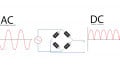
Rectification is a significant part of an electric circuit as it plays a role in converting AC voltage to DC voltage. This article teaches about half-wave rectification, its circuit diagram, waveforms, and analysis.
In electronics, several types of currents exist, of which alternating current (AC) and direct current (DC) are part. Power supply companies feed consumers with alternating currents. Consumers have a variety of devices that operate using AC, for example, AC motors. Others consume DC power, for example, DC motors. For DC gadgets to work, AC power supply needs to be converted to DC power.
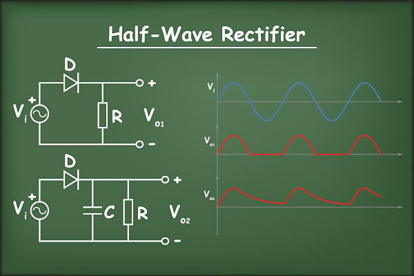
Image used courtesy of Adobe Stock
The process of converting AC to DC is referred to as rectification, and the device that helps in the process is a rectifier. Rectification is classified into two types according to the output characteristics of the rectifier. The two types are half-wave rectification and full-wave rectification. This article focuses on half-wave rectification.
Half-Wave Rectification
Rectification is only performed during the half-cycle process. The alternating current signal is passed through the step-up or step-down transformer, which corrects the voltage to the required level. A step-down transformer often finds more use in the rectifier circuit.
Here, a given input voltage goes through a PN-type junction diode which operates as the rectifier. The PN-junction diode converts AC to DC, which is pulsating. The action is carried out only for the input’s positive half-cycle. At the rectifier circuit's end, the load resistor is connected. Figure 1 shows the half-wave rectification circuit.

Figure 1. The circuit diagram of the half-wave rectification. Image used courtesy of Simon Mugo
How Half-Wave Rectification Works
The supply signal is fed to the step-down transformer (T1), which lowers the voltage at the input. From the transformer, the output is connected to the diode (D1) input which is the rectifier in the circuit. The diode D1 can only get ON during the half-cycle positive input signal where there is current flow in the electric circuit, creating a voltage drop across the output load resistor RL. For the negative half-cycle, the diode D1 gets off and does not conduct; hence, zero current flows through the diode D1, and zero voltage drop occurs at the output load resistor RL.
Waveforms at the Input and Output of the Half-Wave Rectifier

Figure 2. Half-wave rectifier input and output waveforms. Image used courtesy of Simon Mugo
From the waveforms, we can conclude that the output of the half-wave rectifier is a dc that is in pulsation. Let’s analyze the above circuit by working with several parameters, as shown below.
Halfwave Rectifier Analysis
For the analysis, we start with the known equation of the input voltage given by:
\[v_{i}=V_{m}sin\omega t\]
Where; Vm is the supply voltage maximum value.
For an ideal diode, assume: Forward direction resistance is Rf and reverse direction resistance is Rr.
The equation determines the current in RL or diode:
\[i=I_{m}sin\omega t\,\,\,for\,0\leq\omega t\leq2\pi\]
\[i=0\,\,\,for\,\pi\leq\omega t\leq2\pi\]
Where:
\[I_{m}=\frac{V_{m}}{R_{f}+R_{L}}\]
Output DC Current
The average DC flowing in the circuit is determined by:
\[I_{dc}=\frac{1}{2\pi}\smallint\limits^{2\pi}_{0}i\,d(\omega t)\]
Replacing the value of I with the correct formulas and rearranging results in:
\[I_{dc}=\frac{1}{2\pi}[\smallint\limits^{\pi}_{0}I_{m}sin\omega\,t\,d(\omega t)+\smallint\limits^{2\pi}_{0}0\,d(\omega t)]\]
Integrating the equation results in:
\[I_{dc}=\frac{1}{2\pi}[I_{m}\{-cos\omega\,t\}^{\pi}_{0}]\]
Simplifying the above equation:
\[I_{dc}=0.318I_{m}\]
The value of Im and can be substituted with:
\[I_{dc}=\frac{V_{m}}{\pi(R_{f}+R_{L})}\]
If RL >> Rf, then:
\[I_{dc}=\frac{V_{m}}{\pi R_{L}} \]
\[=0.318\frac{V_{m}}{R_{L}}\]
Output DC Voltage
The output DC voltage of the circuit above is determined by:
\[V_{dc}=I_{dc}\times R_{L}\]
But \(I_{dc}=\frac{I_{m}}{\pi}\)
Therefore:
\[V_{dc}=\frac{I_{m}}{\pi}\times R_{L}\]
The value of Im and can be substituted to get:
\[V_{dc}=\frac{V_{m}R_{L}}{\pi(R_{f}+R_{L})}\]
Simplifying this equation, results in:
\[V_{dc}=\frac{V_{m}}{\pi\{1+(\frac{R_{f}}{R_{L}})\}}\]
If RL >> Rf, then the equation reduces to:
\[V_{dc}=\frac{V_{m}}{\pi}=0.318V_{m}\]
RMS Voltages and Currents
For RMS currents, use the equation below:
\[I_{rms}=\sqrt{\frac{1}{2\pi}\smallint^{2\pi}_{0}i^{2}d(\omega t)}\]
Replacing the value of I results in:
\[I_{rms}=\sqrt{\frac{1}{2\pi}\smallint^{2\pi}_{0}I_{m}^{\,\,\,\,2}sin^{2}\omega t\,d(\omega t)+\frac{1}{2\pi}\smallint^{2\pi}_{\pi\pi}0\,d(\omega t)}\]
Replacing with relevant trigonometric the above equation equals:
\[I_{rms}=\sqrt{\frac{I_{m}^{\,\,\,\,\,\,\,2}}{2\pi}\smallint^{\pi}_{0}\Big(\frac{1-coscos2\omega t}{2}\Big)d(\omega t)}\]
Integrating the above equation:
\[I_{rms}=\sqrt{\frac{I_{m}^{\,\,\,\,\,\,2}}{4\pi}\{(\omega t)-\frac{sinsin}{2}\}^{\,\,\,\pi}_{\,\,\,0}}\]
When replacing the limits:
\[I_{rms}=\frac{I_{m}}{2}\]
But we know the formula for Im and replacing it in the formula above results in the RMS current flowing through the load:
\[I_{rms}=\frac{V_{m}}{2(R_{f}+R_{L})}\]
The RMS voltage output across the load is determined by:
\[V_{rms}=I_{rms}R_{L}=\frac{V_{m}R_{L}}{2(R_{f}+R_{L})}\]
Rearranging the above equation results in:
\[V_{rms}=\frac{V_{m}}{2\{1+(\frac{R_{f}}{R_{L}})\}}\]
If RL >> Rf, then the equation results in:
\[V_{rms}=\frac{V_{m}}{2}\]
Efficiency of Half-Wave Rectifier
For the best output, any given electric circuit must be efficient. For the efficiency of the half-wave rectification calculation, take into consideration the output-to-input power ratio.
The formula for the efficiency can be defined as:
\[\eta=\frac{Output\,DC\,Power\,of\,the\,Load}{Input\,AC\,Power\,from\,the\,Transformer}\]
But \(P_{DC}=\frac{I_{m}R_{L}}{\pi^{2}}\,and\,P_{AC}=P_{a}+P_{r}\)
Where:
Pa is the electric power that is dissipated at the diode junction
\[P_{a}=\frac{I_{m}^{\,\,\,\,\,\,2}}{4}R_f\]
And Pr = to the electric power that is dissipated by the load
\[P_{r}=\frac{I_{m}^{\,\,\,\,\,\,2}}{4}R_{L}\]
Therefore:
\[P_{AC}=\frac{I_{m}^{\,\,\,2}}{4}(R_{L}+R_{f})\]
Now efficiency can be shown as:
\[\eta=\frac{4}{\pi^{2}}\frac{R_{L}}{R_{f}+R_{L}}\]
Simplifying and multiplying by 100%, the efficiency formula becomes:
\[\eta=\frac{40.6}{[1+(\frac{R_{f}}{R_{L}})]}\]
Ripple Factor
Even if the rectifier has converted the AC to DC, there is a certain amount of AC left behind in ripple form. For pure DC, one must understand the ripple factor.
Ripple factor is the ratio and can be calculated using the formula below:
\[Ripple\,Factor=\frac{Ripple\,Voltage}{d.cVoltage}=\frac{I_{r(rms)}}{I_{dc}}=\frac{V_{r(rms)}}{v_{dc}}\]
Regulation
The percentage voltage regulation of the half-wave rectification can be determined by:
\[Percentage\,Regulation=\frac{V_{no-load}-V_{full-load}}{V_{full-load}}\]
Transformer Utilization factor (TUF)
The DC power that should be supplied to the load determines which the transformer size that should be utilized in the circuit.
TUF can be calculated as:
\[TUF=\frac{DC\,Power\,for\,the\,Load}{Secondary\,Output\,AC\,rating\,of\,the\,Transformer}\]
Part 2 of this series will focus on full-wave rectification.