Is Spice Modeling Easier the Second Time Around?

This article is published by EEPower as part of an exclusive digital content partnership with Bodo’s Power Systems.

The task of creating models presents numerous challenges for both discrete components and ICs, particularly when working with legacy SPICE software. With discrete components, SPICE doesn’t have built-in device equations for many common discrete components. For ICs, most current modeling methods are cumbersome and time-consuming. The issue is that SPICE was originally intended for IC design and was not specifically designed for using discrete components in circuit simulations.

Discrete Component Modeling

When conceiving and writing Qorvo’s QSPICE, Mike Engelhardt, who also wrote LTspice, made multiple improvements with respect to simulating discrete components such as MOSFETs, JFETs, and diodes. One of his central goals in creating QSPICE was to devise new device equations for these parts that match their performance much more precisely than those in other SPICE software. He also extended the built-in device equations in QSPICE for wide bandgap GaN and SiC MOSFETs and JFETs.

Since SPICE, as originally developed, didn’t include accurate device equations for these parts, modeling challenges emerged. “For example, consider the normal power MOSFET,” Mike Engelhardt noted. “The channel is very short – less than a micron, just like in an IC, but the width of the channel can be a meter wide in order to handle the potentially many amps of current of a power converter.”

Figure 1. This simulation illustrates the ability of QSPICE users to create models for complex parts in C++ to enable the simulation of highly complex circuits, such as this brushless DC motor (BLDC) example. Image used courtesy of Bodo’s Power Systems [PDF]

That’s still a small area that fits on a typical die size. The device equations of the channel are well described by the normal SPICE MOSFET device equations for the monolithic MOSFETs of ICs, but the capacitance between the gate and drain behaves very differently from a monolithic MOSFET. In the monolithic MOSFET, the gate and drain are adjacent

With MOSFETs in ICs, the channel is beneath the gate and doesn’t have a strong impact on the gate-drain capacitance. But the conventional discrete power MOSFET is a vertical device – the gate and drain are opposite each other and form a parallel plate capacitor with the channel between the plates, Mike Engelhardt explained. “For discrete MOSFETs, the channel’s conductivity has a strong impact on the gate-drain capacitance. It’s common for a power MOSFET’s gate-drain capacitance to vary by a factor of five depending on whether the channel is conducting or not. Since this gate-drain capacitance is the Miller capacitance, you can’t present the switching behavior of a normal power MOSFET in SPICE with the built-in device equations. That’s the problem.”

In principle, there would be two ways of solving this problem, he said. One way would be to use the behavioral modeling capability of SPICE to implement new device equations, but this results in wildly complicated models that go on for pages. “The dark side of me finds these models amusing, the mature side of me finds them sad,” Mike Engelhardt continued.

“It’s like someone has an axe to grind because they were rejected from Mensa and wanted to make MOSFET models so complicated no one else can understand or use them.” Such models often crash a SPICE program. “Whereas SPICE can solve a circuit with very many thousands of transistors, it can have trouble trying to solve a circuit with a single such MOSFET modeled in this method. Promoting such a model shows a fairly perfect ignorance of circuit simulation.”

The other way to solve this problem, according to Engelhardt, is to extend the device equations in SPICE itself to manage this nonlinear capacitance. “That’s what we’ve done in QSPICE, which natively handles this non-linear charge. The advantage is that it allows accurate simulation of common power MOSFETs with the robustness required to simulate as many as you want in the same simulation.”

The way SPICE has implemented diode modeling has also been flawed. “For example, consider diode reverse recovery due to charge storage of diffusion capacitance. The standard SPICE equations are for a snap diode. A snap diode is a very useful thing. Given a forward current, there is an amount of charge you have to pull out before the diode turns off. This charge to pull out is proportional to the forward current.”

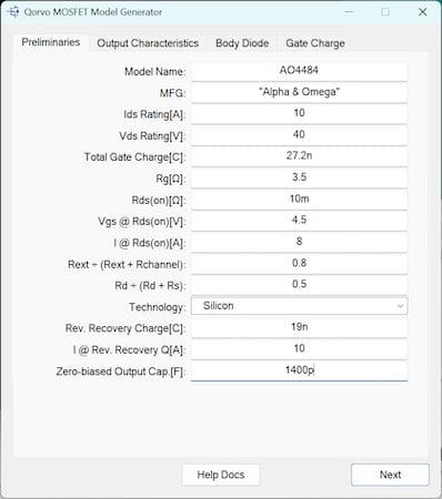
Figure 2. The first step to use the QSPICE Model Generator to create a SPICE model is to plug in basic parameter information from the part’s datasheet. Image used courtesy of Bodo’s Power Systems [PDF]

“Since time multiplied by current is charge, the constant of proportionality has the units of time. This constant of proportionality is the diode model parameter TT, the transient time,” Engelhardt said. “Anyway, a snap diode abruptly goes from conducting to non-conducting in reverse recovery.

With an inductance, you can create an extremely short pulse, like going from zero to a few volts and back in maybe 100 picoseconds. It’s used in particle beam blanking.” But a major SPICE issue for diodes is that most of them aren’t snap diodes, even though every diode in SPICE is a snap diode. “So again, you have to modify the device equations in SPICE to get a diode in simulation to behave as it does in reality.”

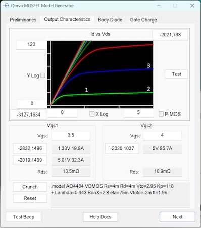
Figure 3. The next step to use the Model Generator is to digitize datasheet curves, in this example, starting with the I_d vs V_DS curves. Image used courtesy of Bodo’s Power Systems [PDF]

JFETs, the red-headed stepchildren of the electronic components world, have always had SPICE issues. “JFETs were never really properly implemented in SPICE,” Engelhardt observed. “In reality, they have a very pronounced quasi-saturation region. Some JFETs go into saturation with a drain source voltage that does not depend on the gate source voltage.”

Historically, no one seemed to care because the production scatter is accepted to be so large, the models for JFETs didn’t make much difference in designs, Engelhardt noted. But QSPICE contains much-improved JFET device equations, and the tool for making discrete JFET models describes much more accurately the performance of these parts in circuits.

The key to improving the model-making process is having a fundamental understanding of the capabilities and limitations of SPICE. Though components such as MOSFETs and JFETs were included in SPICE from the beginning, it was from the perspective of them being within an IC, not as discrete parts. “SPICE has built-in device equations for the devices one can print on an IC,” Mike Engelhardt said. “These are abstract, parameterized equations. SPICE modeling comes down to supplying values for these parameters for a specific instance of a device, and this system works very well for IC design, even for circuits with many thousands of transistors.”

When re-thinking his approach to SPICE while writing QSPICE, Engelhardt started from scratch and addressed some limitations he found while making models for Linear Technology parts. “People know I also wrote LTspice, but what people usually don’t know is I had also made the majority of the IC models in LTspice.” Based on his work creating thousands of LTspice models, Engelhardt made it a priority in QSPICE for designers to be able to build models faster and easier: “Making those mixed signal simulation models was non-trivial. With QSPICE, I solved that problem. One can make detailed models of mixed-signal ICs with minimal effort.”

IC Model Making

The QSPICE embedded library contains a range of model examples useful for creating both simple and complex power ICs. Figure 1 shows a highly complex power management part, the Qorvo ACT72350, modeled in QSPICE using C++.

The C++ used in these examples is fully accessible, which helps designers understand how to create their own models. One example is called PracticalSMPS, in the QSPICE release under File=>Open Demo…=>PracticalSMPS. “It was inspired by an MPS (Monolithic Power Systems) constant on time product,” Engelhardt said. “It only takes a day to make a model like that, and all the behavior is there, including all fault handling. There are also a couple of classic Unitrode parts in the release in their up-to-date form from TI.”

These models are implemented as hierarchical designs so users can look inside and see the proper way to create such models. “You’ll also see some Qorvo devices, and these are literal models of their respective products. Even the SPI and I²C registers are implemented.” He added that if designers want to include SPI or I²C in their own models, it’s quite easy. “There are APIs for both,” he said. “It only takes a few lines of C++ to add them.”

Figure 4. Users can add the curve data using the cursor click technique shown in the “Learn How to Create QSPICE Models in Minutes” video referenced in the article. Image used courtesy of Bodo’s Power Systems [PDF]

Using the Model Generator

A key part of QSPICE’s model-friendly environment is a tool Engelhardt developed that enables users to make their own discrete component models using information typically found on datasheets. This tool is found in QSPICE under File=>Model Generator… =>Diode or JFET or MOSFET.

The Model Generator automates the process of using complex mathematics to transform this data into a SPICE model, cutting the time to make a model from potentially a dozen hours to perhaps a dozen minutes. For more information on modeling discrete MOSFETs, JFETs, and diodes in QSPICE, please visit: https://www.qorvo.com/design-hub/videos/learn-how-to-create-qspice-models-in-minutes

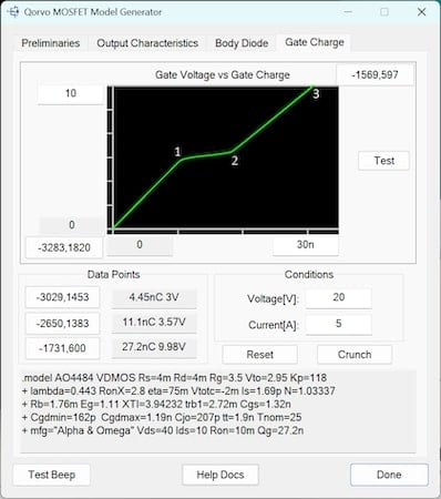
Figure 5. After copying the required curve data into the Model Generator, click “Done” and it performs the calculations and produces a finished QSPICE model for the component. Image used courtesy of Bodo’s Power Systems [PDF]

Creating discrete component SPICE models previously required in-depth knowledge of the physics of electrical component design and the ability to derive parameters using complex mathematical equations. Bob Cordell, a well-regarded circuit design expert, devotes over 30 equation-filled pages to basic SPICE model creation in his recent book, “Designing Audio Circuits and Systems.” An experienced SPICE model engineer might spend a dozen or more hours creating a single model, in addition to time spent collecting data.

In this example, the QSPICE generator is creating a model for the Alpha & Omega Semiconductor AO4484. Users would put basic datasheet information into fields, as shown in Figure 2, to start the model generation process for a particular part. They would then copy curves on the datasheet, Figures 3, 4, and 5, into the QSPICE model generator. The Model Generator performs the calculations and produces a finished QSPICE model for the component:

.model AO4484 VDMOS Rs=4m Rd=4m Rg=3.5 Vto=2.95 Kp=118

+ lambda=0.443 RonX=2.8 eta=75m Vtotc=-2m Is=1.69p N=1.03337

+ Rb=1.76m Eg=1.11 XTI=3.94232 trb1=2.72m Cgs=1.32n + Cgdmin=162p  Cgdmax=1.19n Cjo=207p tt=1.9n Tnom=25 + mfg=”Alpha & Omega” Vds=40 Ids=10 Ron=10m Qg=27.2n

Conclusion

QSPICE has features that simplify the creation of SPICE models for discrete components and ICs while emulating the performance of the parts in circuits more accurately. Fundamental issues with Berkley SPICE and discrete devices are solved in QSPICE through the use of improved device equations. Modeling of complex ICs is made significantly easier through the use of an advanced C++ process. And the addition of a discrete component model generation tool makes the creation of MOSFET, JFET, and diode models vastly easier than with other SPICE software.

This article originally appeared in Bodo’s Power Systems [PDF] magazine.