Facebook
 Google
 GitHub
 Linkedin
Calculating Load Profile
Load profile in power systems determines the approximate energy required by a system over a specific period. In this article, learn how to calculate load profile, the methods involved in the calculation, and solve a practical example.
Power electronic systems consume power. It is the work of the engineers designing the systems to determine how much power the system can consume. Therefore, a smart engineer must be well-equipped to calculate the system's load profile.
Some systems consume too much power while others do not. Most of the systems have power rating tags on them. The ratings are done to describe how the system consumes power at a designated period. The approximation of the power an electrical power system consumes within a specific period is what we refer to as the load profile.
The power system load profile is represented by a rectangular graph showing the instantaneous loads over a particular time. This is the easiest way to study the system's load changes over time. The process of energy load approximation is crucial to designers and engineers as it provides the necessary information to determine the size of energy storing devices because the storage capacity of such gadgets is dependent on the total energy needed to power the loads connected.
Calculating Load Profile
To develop the load profile, two methods are used.
The 24-Hour Method
This method involves the calculation of the average value of instantaneous loads that consume power over the period of 24 hours. The method is preferred when carrying out power utilization for solar systems applications.
Autonomy Method
The method is suitable for backup applications such as UPS and battery systems. The method determines the average instantaneous system loads over a backup/ autonomy time which is the period in which the power loads require backup systems to supply them with electric energy.
The two methods utilize three basic steps with slight differences.
- Develop a list of all the connected loads
- Carry out load profile development
- Carry out the computation of all the total design load and energy required by the system˘¿
Step 1: List of Loads Preparation
This is the first step where all the collected loads are converted into a load list.
24-Hour Method
Here, the time is controlled by an ON and OFF time. The ON represents when the load is turned ON and the OFF represents when the load is turned OFF. For the load systems needed for 24 continuous hours, the ON is represented by 00:00, and the OFF time is represented by 23:59 hours, respectively.
The Autonomy Technique
Here, the period is labeled autonomy which is interpreted to mean back-up, and it is the representation of the total number of hours the load requirements to be supplied with the backup energy such as batteries during the interruption of the service.
Load Consumed Computation (VA)
The formula for calculating the power consumed by the load in Volt-Ampere is below:
\[S_{d}=\frac{P_{d}}{cos\varphi\times\eta}\]
Where
Sd = Apparent power consumed by the load (VA)
\(\eta\)=the efficiency of the load (pu)
Pd = Active power consumed by the load (W)
\(cos\varphi\) = Power Factor of the Load (pu)
Step 2: Load Profile Development
This is developed from the available load list which demonstrates the distribution of the load over a certain period.
Tabulate the loads in the table below by using the Autonomy Method.
|
SECTION |
LOAD IN VA |
AUTONOMY TIME IN HOURS. |
|
Digital Cross Connection |
200 |
4 |
|
Electronic Software Distribution |
200 |
4 |
|
Telecommunication |
150 |
6 |
|
Computer |
100 |
2 |
Table 1. Table of Loads Distribution
To develop the load profile, stack the energy rectangles on top of each other. It is important to note that, in the energy rectangles, height represents the load’s energy, the width represents time, and the rectangle area stands for the total energy of the load. Make sure the broadest rectangle is at the start. The energy rectangle for this problem is shown in the figure below:
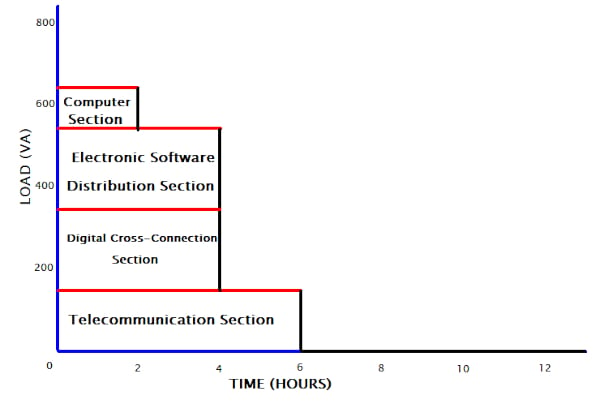
Figure 1. Load Profile
For the 24-hour method, the energy rectangle can be developed using the load period when the load is powered.
Step 3: Design Load and Energy Demand Computation
Design Load
This involves rating all the devices of the systems, such as the breakers, fuses, cables, rectifiers, and inverters. The equation below is suitable for computing the design load:
Sdes = Speak(1+kcont)(1+kdm)
Where:
Sdes = Design Load(VA)
Speak = Peak Load(VA)
kdm = Design Margin in %
kcont = Load growth Contegency Factor in %
During the calculations, engineers should consider the intended future load growth. This has a range of between 5 and 20%. The designers have to take into account unpredicted inaccuracies during the estimations of the load. The design margin has a range between 10 to 15%.
Problem
The pick load apparent power of a system is assumed to be 640VA. By considering that there will be future growth of 10% and the design margin is 10%, calculate the total design load.
Solution
Sdes = Speak(1+kcont)(1+kdm)
parensSdes=640(1+0.1)(1+0.1)
= 774.4VA
Energy Demand
This is utilized while carrying out the energy-storing device sizing. The total energy can only be found by calculating the area within the load profile graph curve.
The total energy can be calculated using the equation listed below:
Ede = Etle(1+kcont)(1+kdm)
Where
Ede = Total Design Energy required in VAh
Etle = Total area under the load profile (VAh)
kdm = Design Margin in %
kcont = Load growth Contigency Factor
Problem
From the table in Figure 1, the total calculated load energy is 2700 Vah. Considering that the future growth will be 10%, and the design margin is 10%, calculate the total design energy required.
Solution
Ede = Etle(1+kcont)(1+kdm)
Ede = 2700(1+0.1)(1+0.1)
= 3267VAh
Key Takeaways of Load Profiles
- Load profile is very important in determining the power consumption of devices.
- Two methods are involved in the load profile calculation: 24-hour and autonomy methods.
- Three general steps have been used in the computation of the load profile
- We have listed all the necessary formulas for load profile calculation.
- We have developed the energy rectangular graphs necessary for load profile calculation.
- We ended the article by solving the load profile problems.
Featured image used courtesy of Adobe Stock