Understanding Capacitance in Overhead Transmission Lines

In power transmission systems, overhead lines feature some electrical properties, which include resistance, capacitance, and conductance along their lengths. Acting as distributed parameter systems, these properties significantly mold the behavior of power in these lines.

The continuous nature and variation of aspects like voltage and current along their path warrant the need for analysis of the behavior of these power lines with distributed parameters.

Parameters like capacitance in overhead transmission lines result from the potential difference between the conductors and the ground or between the overhead conductors themselves. In ultra-high voltage (UHV) networks, the effect of capacitance is more significant as the length of the power line becomes longer.

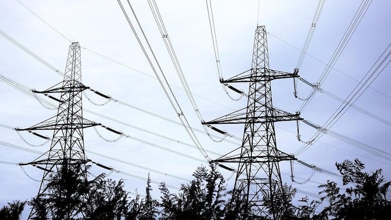
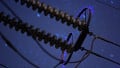
Figure 1. High-voltage transmission lines for long-distance power distribution. Image used courtesy of Pixabay.

In high-voltage AC systems, capacitance in overhead lines can influence voltage regulation by causing the Ferranti effect, making the voltage at the receiving end of the power line higher compared to the voltage being fed to the line.

The potential difference due to this generated capacitance not only causes stress to the insulation of the conductor but also influences the levels of EMI interference. When it comes to managing the reactive power resulting from these capacitances, static VAR compensators (SVCs) or shunt reactors may be needed to support the voltage levels.

Capacitance in Single-Phase Power Lines

Capacitance in two-conductor single-phase AC power lines is greatly influenced by the radius of the conductors and the distance between the conductors. To evaluate the capacitance between the continuous AC power lines, consider the schematic cross-section in Figure 2 showing two conductors with radius r and distance D apart and are suspended off the ground.

In such a setup, an assumption can be made that the conductors are parallel and have uniformly distributed charge. With these assumptions, the capacitors of the power line per unit length of the conductor can be evaluated by first considering the principles of electrostatics, specifically Gauss's law, which offers a basis for understanding how charge distributions and electric fields relate.

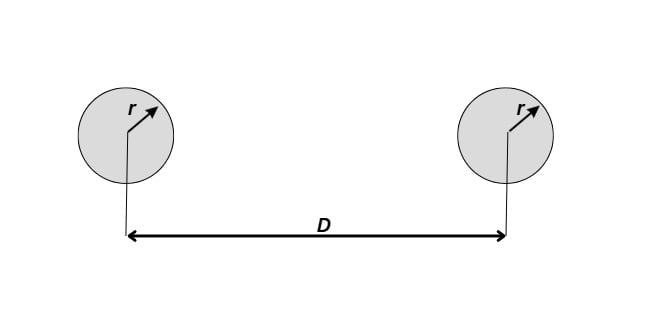
Figure 2. Cross-section schematic of two conductors of single-phase power lines indicating the distance D and the radius r of the conductors. Image used courtesy of Bob Odhiambo.

The first step in deriving capacitance in single-phase power lines is to evaluate the electrical field around a single conductor with a uniform distribution of charge. Consider a straight conductor with charge per unit length (λ = q), the radial electric field from the conductor’s center to a radial distance x, (E(x)) can be evaluated by considering the permittivity (ε₀) of the free space, which is approximately 8.854×10⁻¹² F/m.

$$E(x) = \frac{\lambda}{2 \pi \epsilon_o x}$$

With the evaluation of the electric field, we can now determine the potential difference (V) between the conductors to use in the calculation of capacitance per unit length of the single-phase power lines. The potential difference can therefore be evaluated by integrating the electrical field from the surface of one conductor to a distance (D-r) with symmetry assumption in mind.

$$V = \int_r^D E(x) dx = \int_r^D \big( \frac{\lambda}{2 \pi \epsilon_o x} \big)dx = \big( \frac{\lambda}{2 \pi \epsilon_o x} \big) \ln(\frac{D}{r})$$

The next step is to substitute the potential difference capacitance evaluation formula.

$$C = \frac{q}{V} = \frac{\lambda}{V}$$

Substituting the value of V from the above we can get the overhead line capacitance per unit length of a two-conductor single-phase power line. As the distance between the two conductors increases, the capacitance per unit length reduces due to a weakened field, as illustrated in Figure 3.

$$C = \frac{2 \pi \epsilon_o x}{\ln(\frac{D}{r})} ~[F/m]$$

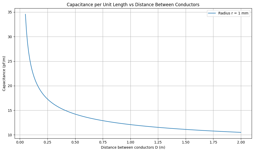
Figure 3. Graph illustrating a drop in capacitance of the conductor per unit length as the distance between the conductors widens. Image used courtesy of Bob Odhiambo. (Click on image to enlarge)

For conductors, an increase in radius distributes the electrical field over a large surface, allowing for an increase in the stored charge. Understanding capacitance in these power lines can help in the implementation of reliable power lines that offer stable voltage transmission without excessive charge currents.

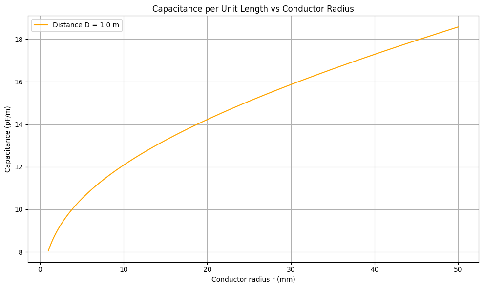
Figure 4. Graph illustrating an increase in capacitance of the conductor per unit length as the radius of the conductor increases. Image used courtesy of Bob Odhiambo. (Click on image to enlarge)

Capacitance in Three-phase Transmission Lines

How conductors are geometrically arranged in three-phase power lines greatly influences the capacitance in the lines. The arrangement of either symmetrical or unsymmetrical conductors determines the approach taken to evaluate the capacitance value.

In a symmetrical three-phase approach, each conductor is subjected to similar capacitive effects as they are arranged in an equilateral triangle, meaning distance D is the same as shown in Figure 5.

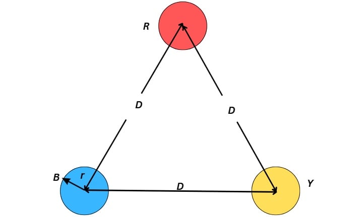
Figure 5. Equilateral triangle three-phase conductor layout showing spacing (D) and the radius of the conductor (r). Image used courtesy of Bob Odhiambo.

Each phase in the symmetrical arrangement can be paired against the neutral and the capacitance per phase to neutral be evaluated just like in a single-phase power transmission line.

$$C_{phase} = \frac{2 \pi \epsilon_o}{\ln(\frac{D}{r})} ~[F/m]$$

Unlike symmetrical three-phase conductors, unsymmetrical conductors exhibit unbalanced phase angles and inconsistent capacitance levels. Therefore, a geometric mean distance (GMD) needs to be evaluated to determine the actual spacing between the conductors.

To ensure consistency in the electrical properties of the transmission lines, the conductors are swapped periodically from their initial position so that each one occupies each of the three possible positions for one-third of the power line’s length. As a result, each phase experiences uniform characteristics, ensuring a balanced three-phase system despite not being symmetrical.

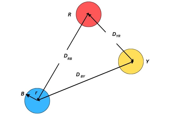
Figure 6. Unsymmetrical arrangement of three-phase conductors, showing the different spacing lengths between the conductors and the radius of the conductor (r). Image used courtesy of Bob Odhiambo.

Considering Figure 6, for instance, we can first determine equivalent spacing (D_eq) by evaluating the GMD of the conductors.

$$D_{eq} = (D_{RB}~\cdot~D_{BY}~\cdot~D_{YR})^{\frac{1}{3}}$$

The capacitance in unsymmetrical three-phase conductors can therefore be expressed as:

$$C_{phase} = \frac{2 \pi \epsilon_o}{\ln(\frac{D_{eq}}{r})} ~[F/m]$$

Effects of Earth on Transmission Line Capacitance

Other than factors like the distance between conductors or their radius affecting electric field distribution, the presence of earth under high voltage transmission lines that run for long distances also influences the distribution of these electrical fields and hence changes the capacitance values.

The ‘method of images’, a concept from electrostatics, is used to understand the interaction of ground and capacitance. This method replaces the ground plane with an ‘image’ charge to mirror the actual behavior of the overhead conductors.

Assuming a high voltage conductor is placed at ‘h’ distance above the ground levels, its image conductor will be positioned at '–h' with an opposite charge to create a ground surface with zero potential.

The Earth’s presence distorts the electric field lines, increasing capacitance as without the earth, these electric fields will otherwise extend outwards from the conductor in all directions. By employing the concept of images, we can express the capacitance per unit length of a single overhead conductor as:

$$C = \frac{2 \pi \epsilon_o}{\ln(\frac{2h}{r})} ~[F/m]$$

In power lines carrying low voltages, the earth's effect on the capacitance is negligible. However, in high-voltage transmission lines, earth effects account for a 10-30% increase in capacitance levels, influencing aspects like charging currents and voltage drops.

Engineers can therefore consider the earth's influence on capacitance when managing reactive power in distribution lines, sizing shunt reactors, and designing electrical insulation materials. Meanwhile, factoring in the other aspects mentioned in the article that influence capacitance ensures efficiency and accuracy in designing transmission lines.