Facebook
 Google
 GitHub
 Linkedin
ONE Design Equation for Custom Inductors An Introduction to Power Electronics
Over 35 years ago, I started my career in power electronics. I completed a practical power project in my senior year in college, building a 6KV, 20kHz
Over 35 years ago, I started my career in power electronics. I completed a practical power project in my senior year in college, building a 6KV, 20kHz AC output power supply. It was a crash-course introduction into the world of power and set the course for my career. Pushing power through a transformer where nothing on the primary touched anything on the secondary seemed like magic, and I was hooked.
After university, my first interviews were with computer companies in the Boston area, and I really thought that my future was in logic design. However, as interviewers learned that I knew something – anything! – about magnetics and power supply design, I was shunted off to the power department.
In those days, switching power supplies were just beginning to take over the computer industry, and there was a desperate need for design expertise. My first officemate became my mentor — a wonderful man named Spriadon (Dan) Balulescu. On my first day on the job, he put Dr. Cuk’s dissertation on my desk and asked me to explain it to him in a couple of days, I think to prove that I was worthy of his time.
Soon after, we embarked on a 1kW full-bridge power supply for a minicomputer. There was little guidance. FETs were just becoming practical, and there were no current-mode control chips.
I took on the job of simulation, electronics and control design, and Dan did the magnetics design, thermal, and layout. He would work for days at a time on the magnetics, huddled over a notebook, and a working specification would emerge to send off to our vendor. A few weeks later, samples would return. We placed them in the circuit to determine what worked and what didn’t. Two iterations were usually enough to get the job done properly.
Throughout the process, over a period of two years, magnetics design remained a mystery to me. It was the domain of the older, experienced engineers and the magnetics companies. Dan promised me that he would give me all his notes when I left the company to return to graduate school. He was good to his word, but I was no more enlightened after reading them than I was before.
Graduate School and Magnetics
After working for a few years on products at my first job, I went back to graduate school to study under Dr. Fred Lee at Virginia Tech. Dr. Lee had already built a reputation for hiring the best in the world, and I was honored to be included in his group. All graduate students were assigned projects for industry. I was given two – analysis of parallel power converters for IBM, and power converter design optimization for NASA. The NASA project involved writing nonlinear optimization code with Lagrangian multipliers to get to an optimum solution for the selection of power parameters.
This is where I was first exposed to the inner workings of the magnetics design. The nonlinear optimization code worked to move parameters around (switching frequency, core sizes, etc.) to try to find a minimum objective function. In this case—the weight of a converter. The power loss in components was penalized by the weight of a required heatsink. There were many calculations to estimate the performance of the design, but I found something remarkable at the center of the code. There was only ONE equation that had to be obeyed to make magnetics work.
This was a revelation to me – ONE equation? How could that be? Why did magnetics books make it so complicated? They all had this equation but quickly moved on to discuss hundreds more. I posed the question to everyone in the research group at Virginia Tech. Did they know that there is only one equation for magnetics? Everyone was puzzled. They each had a methodology, but could not describe the process.
ONE Equation
Figure 1 shows the basic structure of a generic core with a winding. This shows everything you need to build a custom inductor. The core can be any shape, with any cross-section — square, rectangular, round, or some other shape. The core material sets the permeability, and the ability to open a gap allows adjustment in the permeability of the structure. The gap can also be embedded in the material, but this is a more specialized case for future discussion. There are negative consequences that come with the pre-gapped core material, along with some advantages. For peak performance, the inductor will be a gapped ferrite in most cases.
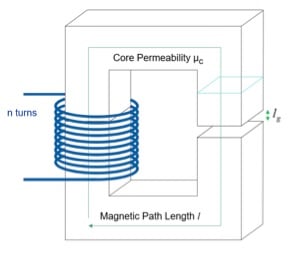
Figure 1. The basic constituents of a custom-designed inductor
There are a lot of design freedoms offered by this structure – core size, number of turns, wire size, permeability, and gap. But where to start with a design? We can look at the basic magnetics equations to decide. The inductance of the structure is given by:
![]()
The area and the path length are shown in Figure 1. The effective permeability of the core, µ, is given by:

We don’t have any idea how to deal with the permeability at the outset. It is very variable in the core with a wide tolerance in the specification. We will control this later with the gap in the core.
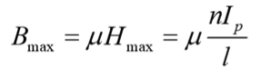
The maximum excitation, H, is given in terms of the peak current in the inductor by:
![]()
The maximum flux of the core is then:
But we do not know how to select any of these variables. So, we do some math tricks:
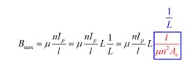
Which leads to several convenient cancellations in the equation:
![]()
Now we have our one equation that matters, and it is independent of the µ of the structure, and the path length l. In fact, for a given saturation level of material, we are left with just two design variables – the area of the core, and the number of turns. The terms on the right of the inequality are electrical variables that we should already know from the simulation of the converter.
![]()
We have three important magnetics parameters now – the area of the core, number of turns, and the maximum B field that is allowed. For any given core, the area is fixed. If you choose a ferrite, the saturation level is also a constant, as we will discuss later.
Core Area
With few variables involved in the design, the type of core (or core shape) becomes irrelevant. Figure 2 shows several different types of cores – EE, RM, EPC, and pot cores. The only parameter we care about is the area. All core types are then treated the same, and the choice of the family is determined by the desired profile, available bobbins, ease of winding and other similarly practical considerations.
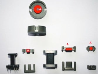
Figure 2. Different core shapes and areas
Inductor design is all about energy storage, determined by the inductance and peak current. We can choose any core, see how many turns are needed, and iterate designs to quickly arrive at a good solution. Only one rule is needed – obey the single equation.
Saturation Level for Ferrites
We need to know the saturation level for ferrites. This level must not be exceeded, or the inductor will drastically drop in value. Figure 3 shows the saturation curves for some TDK parts. Experienced designers will immediately know how to read these curves. The “knee” of the curve occurs around 0.3 T. This is the value used by almost all commercial designs. At 0.3 , there is a small decrease in the Al value for the material. The gap in the core will make this drop undetectable, and the inductor will be constant up to 0.3T
Aerospace companies tend to design more conservatively. They will use a value of 0.25T, or sometimes 0.2T, to provide plenty of design margin.
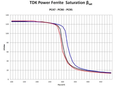
Figure 3. The saturation level of ferrite material. Experienced engineers work with a value of 0.3T for conservative designs.
The 0.3 T level for saturation of ferrites has been well known for years. However, newcomers to the field tend to look for specifications from the manufacturer, as they have not learned to interpret the curves. Unfortunately, this approach can lead to trouble in the design. The core manufacturers typically do not consider the knee of the curve to be the saturation flux. As you can see in Figure 4, they are extremely optimistic about the value of saturation, quoting numbers from 0.38 T to 0.54 T. Using this number for design can lead to failure.
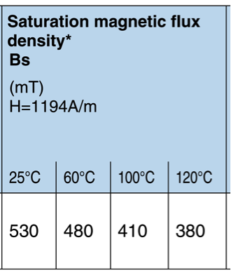
Figure 4. Manufacturer’s specification of the saturation level of ferrite materials. The numbers exceed the value that experienced designers would read from the knee in the magnetization curves.
It is highly recommended to use the curves to derive a comfortable number without exceeding the value of 0.3T — unless the full data of the core material under all extremes of temperature is studied. Even then, exceeding 0.35T is never recommended.
Just One Equation
One design equation is needed for creating inductor designs. Magnetics design is then reduced to a few simple variables. This equation is common in all magnetics books but is not highlighted as the ONE equation that is essential.
Our suggested approach is to use this equation, and then iterate designs to rapidly build experience in inductor design. When choosing a value of saturation flux for design, make sure that you read the curves and do not just accept overly optimistic values provided by core vendors.
References
Magnetics design videos and articles can be found in the Ridley Engineering Design Center.
RidleyWorks Simulation software contains complete magnetics design and advanced analysis.
Learn about proximity losses and magnetics design in our hands-on workshops for power supply design. (This is the only hands-on magnetics seminar in the world.)