Facebook
 Google
 GitHub
 Linkedin
Introduction to Transmission Line Modeling for Power System Analysis
This article series explores the modeling of short, medium, and long transmission lines for reliable simulation of power flow, voltage behavior, and system stability.
In this two-part series, we will explore the classification and modeling of transmission lines based on their length and voltage level. This first article will provide the basic framework by explaining how accurate line models impact power system analysis.
You will learn the importance of incorporating series impedance, shunt admittance, and distributed parameters in the transmission line models. We will then apply this to short transmission lines. The next article will examine the models for medium and long transmission lines.
Role of Transmission Line Modeling in Power Systems
Transmission lines are the physical backbone of any interconnected power system, responsible for transporting electrical energy over long distances from generation sites to load centers. The accurate modeling of these lines is essential for conducting reliable power flow analysis, transient and dynamic stability studies, protection coordination, and system planning.
Inadequate or oversimplified modeling of line parameters—especially over extended distances—can lead to serious misestimations in voltage profiles, power losses, line loading, and even lead to failures in stability margins or protection coordination.
Unlike distribution systems where lumped parameters can often suffice due to shorter distances and lower voltages, transmission systems—especially extra high voltage (EHV) and ultra-high voltage (UHV) networks—require a detailed and distributed treatment of electrical parameters such as resistance (R), inductance (L), capacitance (C), and conductance (G). The correct representation of these parameters in simulations directly influences the system operator’s ability to evaluate system performance under both steady-state and transient conditions.
Classification Based on Line Length and Voltage Level
In power system analysis, transmission lines are typically classified into short, medium, and long lines, based on the line length and the corresponding significance of distributed parameters:
| Line Type | Typical Length Range | Modeling Approach | Voltage Level |
| Short | < 80 km | Series impedance (R + jX) only | Mostly 33–132 kV |
| Medium | 80–250 km | Lumped π or T model | 132–230 kV |
| Long | > 250 km | Distributed parameter model | 345 kV and above (EHV/UHV) |
Table 1. Modeling approach as a function of line length
For short transmission lines, the shunt capacitance between conductors and ground is often negligible and excluded from modeling. However, medium lines require representation of charging currents due to the presence of shunt admittance, typically modeled using nominal π or T circuits. In contrast, long transmission lines must consider the distributed nature of R, L, C, and G along the entire line length, resulting in the need to solve transmission line differential equations that yield hyperbolic voltage and current profiles.
Impact on Design, Stability, and Fault Analysis
The consequences of inaccurate modeling can be profound. For example, neglecting line charging can lead to incorrect voltage estimations at the receiving end in lightly loaded conditions—a classic manifestation of the Ferranti effect. Similarly, in dynamic studies, improperly modeled long lines can distort system oscillation frequencies and damping ratios, resulting in misleading conclusions about system stability.
During fault analysis, especially in distance protection schemes, the accuracy of line impedance directly affects zone settings and reach calculations, potentially leading to overreach or underreach in relays.
Moreover, for HVDC back-to-back interconnections or renewable energy corridors where long HVAC transmission is used, detailed line modeling becomes essential to coordinate protective relays, set appropriate under-voltage load shedding schemes, and implement voltage support systems like synchronous condensers or FACTS devices.
For extremely long lines or lines feeding weak systems (low short-circuit ratio), longitudinal voltage drop, charging currents, and surge impedance loading (SIL) all play significant roles in determining whether reactive compensation is needed to maintain system stability and voltage regulation. All these considerations make rigorous transmission line modeling not just a theoretical necessity but a practical one.
Short Transmission Line Model (< 80 km)
In power system analysis, short transmission lines are generally defined as those with physical lengths under 80 kilometers and operating at voltages in the range of 69 to 132 kV. Due to their limited physical extent, the shunt admittance—primarily the capacitive coupling between the conductors and ground—is considered negligible. This allows the line to be modeled using only lumped series impedance, without introducing substantial error in steady-state power flow or voltage profile analysis.
In this approximation, the transmission line is represented by a single impedance element Z = R + jX, where:
- R is the total resistance of the line, primarily due to conductor material and temperature
- X = ωL is the inductive reactance of the line, which dominates in most overhead systems
This simplified model assumes that the line behaves as a passive series element with no capacitive charging effect. The load at the receiving end determines the current, and the voltage drop across the line is computed directly via Ohm's Law:
$$V_s = V_r + IZ = V_r + I(R + jX)$$
where:
- Vs is the sending-end voltage (complex phasor)
- Vr is the receiving-end voltage (complex phasor)
- I is the line current (also a complex phasor)
This linear relationship allows easy calculation of voltage drops and losses under various load conditions. The real power loss in the line is derived from Joule’s law:
$$P_{loss} = I^2R$$
Given the absence of shunt elements, the line current is solely determined by the load current at the receiving end. Therefore, there is no need to solve for multiple node voltages or charging currents, as is the case in longer or higher-voltage lines.
The short line model is particularly suitable for rural distribution feeders, sub transmission networks, or industrial interconnects, where the line length is sufficiently short that the voltage rise from capacitive charging is insignificant.
However, applying this model beyond its valid range—especially above 80 km or for voltages exceeding 132 kV—can lead to underestimation of receiving-end voltages due to ignored shunt capacitance and Ferranti effect.
An important implication of the short line model is that it cannot capture resonant interactions, surge propagation, or overvoltage conditions associated with long lines. It is strictly a steady-state approximation useful in load flow studies, protection coordination, and basic thermal loading checks, where line charging is not a significant factor.
While the impedance values are often calculated using conductor tables or empirical data, standard per-unit system conversions are applied to normalize these parameters, facilitating comparison across various voltage levels and configurations.
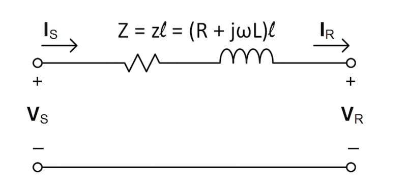
Figure 1. Short transmission line model. Image use courtesy of Oregon State University
Example Calculation
If a 50 km line has an impedance of 0.2 + j0.4Ω/km, the total line impedance is:
$$Z - (0.2 + j0.4) \times 50 = 10 + j20 \text{ }\Omega$$
For a load current of 100 A at 0.9 lagging power factor, the voltage drop becomes:
$$\Delta V = IZ =100 \angle -25.84 ^{\circ} \times 10 + j20$$
Such calculations illustrate how this model remains computationally tractable and analytically intuitive.
Key Takeaways
Accurate modeling of transmission lines is critical for ensuring reliable and efficient power system operation, particularly as modern grids become more complex and sensitive to stability margins, voltage regulation, and fault dynamics. These models directly influence load flow accuracy, protection coordination, and the design of reactive compensation and control strategies.
In practical terms, they are essential for tasks such as setting relay zones, simulating transient behavior during faults, evaluating the Ferranti effect, and planning EHV/UHV corridors for renewable integration.
Countinue reading this 2-part article series with Part 2: Modeling Medium and Long Transmission Lines for Power System Analysis.
Featured image used courtesy of Adobe Stock (licensed)