Model-Based Power Converter Design Using High-Confidence MOSFETs

This article looks at how the power converter designer can use the system-level and detailed models together to enable exploration of the design space and also achieve high confidence in the results. An example of this process will be shown using MathWorks system-level modeling tools Simulink® and Simscape™ with detailed SPICE subcircuits representing Infineon Automotive MOSFETs.

 

Design Questions

During the development of electrical power converters, numerical simulations are typically used during the concept and feasibility study. The simulation models need to include both the analog circuit and the corresponding digital controllers. Examples of the design questions that models can help answer include:

Which topology should be used?

• For a given topology, what performance can be achieved?
• What PWM switching frequency should be used?
• What values and ratings are required for the passive components?

What kind of power switch should be used?

• type (like MOSFETs or IGBTs or BJTs)?
• technology and voltage ratings (like Infineon’s OptiMOS™ or CoolMOS™) and materials (like Si or SiC or GaN)?

What are the requirements on the gate driver circuits including minimum required dead-time?

Finally, based on previous assessments:

• System efficiency and component losses may be estimated, and, subsequently, a suitable cooling system can be developed
• The trade-off of system efficiency with EM compatibility can be investigated. Switching losses and EMI are both dependent on switching frequency and power switch slew rate.

SPICE simulation tools are the go-to solution for circuit designers. However, the design steps described depend on being able to simulate the power converter in a reasonable time. Circuit simulation tools like Simscape™ Electrical™ have simple device models that are essentially ideal switches plus tabulated switching losses that meet this efficient simulation need. Moreover, tight integration with Simulink® means that the digital controller is also included in the simulation with no need for co-simulation. However, the ideal switch assumption creates some uncertainty for the later design steps focused on determining efficiency and fine-tuning the design. This uncertainty can be addressed by using detailed SPICE device models developed by the component manufacturer. In this paper, a process is defined that enables fast exploration of the design space whilst also capitalizing on the detailed foundry SPICE component models. Central to the process is making use of multiple models with differing levels of fidelity, matching the model to the specific design question to be answered. Also important is the use of low fidelity levels to pre-initialize detailed simulation models thereby reducing initialization time.

 

Buck Converter Design Example

A 48V/12V DC/DC step-down buck converter shown in Figure 1 is used as an example in this paper. A buck converter steps down the input voltage (V_IN) to a lower-level output voltage (V_OUT), and the main equation characterizing its behavior is given by:

Equation 1

\[d=\frac{V\_OUT}{V\_IN}\Rightarrow V\_OUT=d\,*\,V\_IN\]

where d represents the duty cycle of the high side power switch (HS_SW). The duty cycle of the low side power switch (LS_SW) is given by d’ defined by:

Equation 2

d' = 1 − d

 

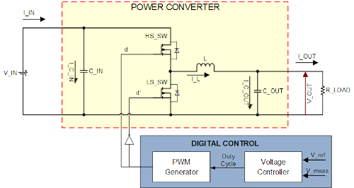
Figure 1. Structure of buck (Step-Down) DC/DC power converter. Image used courtesy of Bodo’s Power Systems

 

Based on the reference voltage (V_ref) and measured output voltage (V_meas), the discrete-time proportional plus integral voltage controller calculates the required duty cycle (d).
 

Infineon SPICE MOSFET model

SPICE (Simulation Program with Integrated Circuit Emphasis) simulators are the most commonly used technology for analog circuit simulation. Therefore, as a de-facto industrial standard, many semiconductor manufacturers develop SPICE models of their products to support circuit design.

Infineon’s portfolio of automotive qualified OptiMOS™ power MOSFETs offers benchmark quality in a range from 20 V-300 V, diversified packages and an R_ds(on) down to 0.55 mΩ. The structure of Infineon’s SPICE model of MOSFET is shown in Figure 2. This behavioral MOSFET model [1] describes both the electrical and thermal characteristics of the power switch.

 

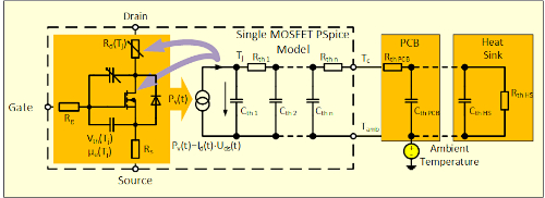
Figure 2. Schematic of Infineon's SPICE MOSFET model structure. Image used courtesy of Bodo’s Power Systems

 

The model reflects that current flowing through the MOSFET causes changes in semiconductor temperature which, in turn, influences the MOSFET electrical parameters such as charge carrier mobility, voltage threshold, drain resistance, gate-drain capacitance and gate-source capacitance. Referring to Figure 2, thermal behavior is modeled in the following way: a current source (P_v) representing MOSFET dissipated power injects the heat into the PN-junction (T_j ), and that heat is then propagated all the way through MOSFET package to the case (T_c). The thermal dynamics is modeled as a Cauer network made up of lumped thermal resistances (R_thi) and thermal capacitances (C_thi). By means of analog simulation of the thermal model, the optimum cooling/heat sink (R_{th HS} and C_{th HS}) can be determined for given design parameters like load current, maximum allowed junction temperature (T_j ), ambient temperature (T_amb) and thickness/number of PCB layers (R_{th PCB} and C_{th PCB}).

 

Importing a Subcircuit into Simscape

Simscape [5] from MathWorks provides a block diagram environment to model multi-domain systems, including electrical, mechanical, magnetic and thermal aspects. The accompanying Simscape language expresses the underlying physics using differential equations, associated algebraic constraints, events and mode charts.

 

Figure 3. Infineon’s Automotive MOSFET IAUT300N08S5N012 in TOLL (PG-HSOF-8). Image used courtesy of Bodo’s Power Systems

 

Simscape Electrical™ [6] is able to import a targeted set of SPICE device models, such as MOSFETs, into an equivalent Simscape language implementation [7]. Simscape’s tight integration with Simulink then enables simulating both the digital controller and the analog electronics with a single solver, resulting in a more efficient simulation than co-simulation between different simulation tools.

The SPICE model import capability is used to import the Infineon IAUT300N08S5N012 [2][4] device (shown in Figure 3) into Simscape. Once imported into Simscape, some minor edits were made to the Simscape code to provide access to the Cauer model states from the published block. Providing customized access to the internal states is needed for the initialization process.

 

Simulation Workflow

Having imported the Infineon device into Simscape, the next step is to create a Simulink model of the complete converter including the imported Infineon devices, remaining analog components and the controller. This is shown in Figure 4.

The controller is implemented using Simulink discrete-time library blocks, and the complete model is simulated using a variable-step solver so that the faster time constants associated with parasitics and the MOSFET charge model are accurately captured. The simulation time for one controller PWM cycle is 2.3 seconds on an Intel® Core™ i7-9700 CPU @ 3.00GHz running MATLAB version R2021b. This is fast enough to analyze circuit performance at the current operating state, but not to assess circuit sensitivity to design parameter sweeps or to directly optimize the circuit parameters. Furthermore, it is not fast enough to simulate a periodic steady-state which, given a thermal time constant of approximately 10 seconds, equates to 200,000 20kHz PWM cycles.

 

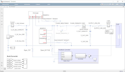
Figure 4. Detailed model of the buck converter. Image used courtesy of Bodo’s Power Systems

 

To address the need to explore the design space efficiently, a system-level version of the buck converter model was created. For this, the imported MOSFET device models are replaced with ideal switches with fixed on-resistance set to the datasheet R_ds(on) value. This is shown in Figure 5. Some of the faster parasitics are also omitted, such as the MOSFET lead inductances. This system-level model is fixed temperature, the user setting an appropriate R_ds(on) value for the assumed junction temperature. The model takes around 0.05 seconds to simulate one PWM cycle, 46 times faster than the detailed model. As there are no thermal time constants, the slowest dynamic is now associated with the voltage regulation and is of the order of 5ms or 100 PWM cycles. Simulation to steady-state takes approximately 5 seconds.

With this simulation performance, the system-level model can be used to thoroughly explore the design space and optimize the controller. With the main design decisions made, the final step is to validate the design using the detailed simulation model that makes use of the Infineon MOSFET models. This validation is typically reported at a set of operating points defined by load power and ambient temperature. However, we have seen that simulating the detailed model to steady-state requires 200,000 PWM cycles which is not practical if each cycle takes 2.3 seconds to simulate.

 

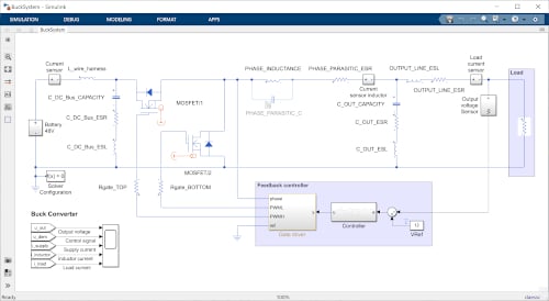
Figure 5. System-level Simulink model of the buck power converter. Image used courtesy of Bodo’s Power Systems

 

To initialize the detailed model at a specified operating point, an iterative approach involving multiple models is proposed. Overall, the idea is to separate out slower time constants into separate models that run faster. Before explaining in more detail, one more model is required which is one that models the MOSFET and environment thermal states only. This is shown in Figure 6.

To construct the thermal-only model, the imported Infineon SPICE subcircuits are edited to leave just the Cauer network. The input to the two Cauer networks is two constant heat flow sources Q1 and Q2 which represent the average junction heat flow per PWM cycle. This thermal-only model can either be run to steady-state, or the Simscape start from steady-state option used. Either way, the time to solve the Cauer network node temperatures is negligible compared to everything else.

 

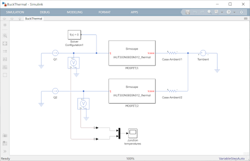
Figure 6. Simulink thermal only model of the two MOSFETs. Image used courtesy of Bodo’s Power Systems

 

The three models are now used to initialize the detailed model in periodic steady-state as follows:

1. Run the System-level model (Figure 4) to periodic steady-state. Average the MOSFET losses over the last full PWM period to give estimates for the junction losses, Q1 and Q2.
2. Run the Thermal-only model (Figure 6) to thermal steady-state and record the final temperatures for the nodes of the two Cauer models.
3. Set the Detailed model’s (Figure 5) thermal states equal to the values from Step 2 above, and set the remaining model states to the values determined from Step 1 above.
4. Run the Detailed model for four complete PWM cycles. Average the MOSFET losses over the last full PWM period to give revised estimates for the junction losses, Q1 and Q2.
5. Repeat Step 2 to revise the thermal node temperatures.
6. Repeat Step 4 to revise the initial states and junction losses estimate.

Steps 5 and 6 can be repeated if needed, but for this example, this was not necessary. The model is now sufficiently close to a periodic steady-state, and circuit performance can now be assessed.

Figure 7 shows the instantaneous switching losses when powering a 2.85kW load, plus the overall converter efficiency. This level of efficiency is on the low side, and the designer’s next step might be to implement two or three MOSFETs in parallel for both the high-side and low-side switches. The important thing to note is that there can be a high level of confidence in this result given that the validated foundry SPICE MOSFET models were used to generate them and that the results are for the actual circuit. This gives a higher level of confidence than the sometimes-used alternative based on datasheet plots of on-state and switching losses for a representative test circuit.

 

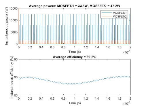
Figure 7. Losses in power switches and efficiency of overall system. Image used courtesy of Bodo’s Power Systems

 

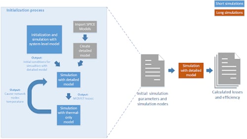
Figure 8. Proposed simulation flow for switching power converters. Image used courtesy of Bodo’s Power Systems

 

A summary of the overall process followed is shown in Figure 8. The process is implemented as a MATLAB® script which can be downloaded from MathWorks File Exchange [3]. The script takes four minutes to run and produce the results in Figure 7. For comparison, it was determined that running the non-linear model from a non-initialized state to get the same results takes on the order of a day.

 

Conclusions

It has been shown how detailed SPICE foundry semiconductor models can be used in an application circuit model to make high-confidence predictions about expected circuit performance. The challenge of initializing a model with widely varying time constants and with a periodic steady-state has been tackled with a two-pronged approach. First, avoidance of slow co-simulation is achieved by importing SPICE subcircuits into Simulink, and solving the complete analog system plus controller using a variable-step solver. Second, the steady-state is found by using multiple models with different fidelity levels with a simple iterative scheme. The end result is an end-to-end design and simulation capability that is faster than if working solely with a SPICE simulation engine.

 

This article was co-authored by Radovan Vuletic, Infineon Technologies, and Rick Hyde, MathWorks, and originally appeared in Bodo’s Power Systems magazine.