Determining Semiconductor Chip Temperature

This article is published by EEPower as part of an exclusive digital content partnership with Bodo’s Power Systems.

The semiconductor’s temperature development is the most important factor determining a power-electronic system’s service life. For this reason, it is very important to determine the chip temperature as accurately as possible.

All datasheet specifications and service life calculations refer to a mathematical construct of a virtual chip temperature or virtual junction temperature T_vj. Determining a power semiconductor’s temperature is not a trivial task. This is because, strictly speaking, there is no such thing as “chip temperature.”

In-Situ

The so-called in-situ measurement is the method of choice for measuring chip temperature in the laboratory. Here, the chip to be measured is first heated to precisely defined temperatures using a calibrated heating plate. A small measuring current is injected, and the resulting forward voltage is measured. A linear relationship exists between the forward voltage and the chip’s temperature, providing a constant and precisely known current flows.

The current must be small enough not to contribute to heating the semiconductor but large enough to generate measurable voltage. Values around 1% of the nominal current of the semiconductor to be tested have proven reasonable. In turn, the chip temperature can be determined from the correlation, which is unique and reversible if the previously used current is used and the voltage on the component is known.

The result of this laboratory measurement is based on a constant chip temperature, and due to the external heating, the chip has a homogeneous temperature distribution. This special case, which does not reflect the conditions in the real application, provides “the chip temperature” or the “junction temperature” T_j.

Real-World Applications

In the real application, however, there is a temperature gradient across the chip’s surface; the chip is hotter in the center than at the edges, especially at the corners. This is because more heat can be transferred to the surrounding assembly and connection technology at the edges and corners than in the center of the chip.

The effect can be seen in measurements such as those in Figure 1, which are taken using an infrared (IR) imaging camera.

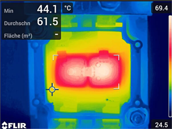
Figure 1. IR image of two diodes connected in parallel under DC load. Image used courtesy of Bodo’s Power Systems [PDF]

Alternatively, a sensor placed on the chip, such as a type K thermocouple, is often used. Although the sensor then provides a temperature value, this does not necessarily represent the value required for characterization and service life determination. One advantage of this measurement is that it is possible to measure during operation at high voltage and current, provided the measurement equipment meets the requirements for protecting equipment and personnel. This is important as the sensor is in galvanic contact with the chip and carries a potentially lethal voltage.

The temperature sensor is often placed in the center of the chip to reliably deliver the maximum value. If the thermal relationships are known precisely enough, conclusions can also be drawn from the maximum value to the average value.

The virtual chip temperature T_vj, representing an average temperature value over the entire chip surface, is always of interest when considering the service life and thermal design. If it can be implemented, the in-situ measurement also precisely provides this value in the real setup, as only one voltage at one current needs to be measured. Averaging is an inherent part of this measurement setup. The measured voltage represents the chip temperature as if it were homogeneously distributed.

Reliability Tests

Reliability tests at semiconductor manufacturers are monitored using the in-situ method. Here, the approach is close to the application as the chip is actively heated. The information on load cycling resistance based on this method already includes the fact that the maximum temperature value on the chip is higher than the specified temperature. This approach is conservative and ideally suited to characterization measurements and quality assurance processes.

Another way to calculate the mean value is by evaluating IR images. This method also allows the observation of semiconductors in real operation and provides precise and application-related information. For evaluation, the software belonging to the IR camera usually allows an area of interest to be defined and the correlating mean value within it to be determined. This procedure is used in Figure 1; the area under consideration comprises two diodes connected in parallel.

The disadvantage of this method is that the observed semiconductors must not be potted. Even if they are optically transparent, potting compounds block the emitted infrared radiation, making this way of measurement impossible. Consequently, such setups cannot be operated with high voltages because the lack of insulation can lead to arcing, malfunction, and even destruction.

A frequently used alternative evaluation consists of determining the temperature T_M in the center and the temperature T_E in one corner of the chip and performing a 2-to-1 weighting.

The virtual chip temperature results in T_vj=1/3·(2·T_M+T_E). This is possible from both the IR image and using two correctly positioned temperature sensors.

It is no coincidence that even this seemingly simple method delivers accurate values. The precision can be explained by the thermal conditions along the chip diagonals.

From one corner to the diagonally opposite corner, the temperature across the chip develops along a dome-shaped curve. A good approximation of this shape is a parabola or a sinusoidal curve. Due to the simple relationships, the sinusoidal curve is preferred here.

The mean temperature results from the effective value of the sine curve and the offset. Figure 2 depicts the curve that can be assumed in this case.

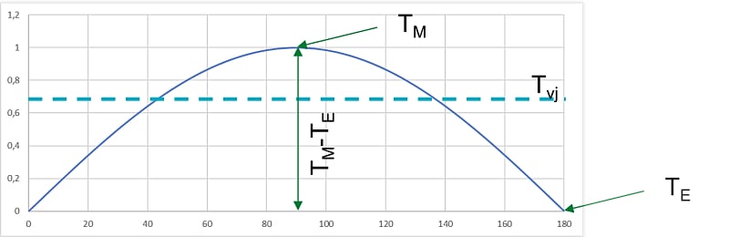
Figure 2. Temperature distribution along the diagonal of a chip. Image used courtesy of Bodo’s Power Systems [PDF]

The required mean value corresponds to the RMS value, which is calculated from the amplitude (T_M-T_E) and the offset T_E as

\[T_{eff}=T_{vj}=\underbrace{\frac{1}{\sqrt{2}}(T_{M}-T_{E})}+T_{E}\leftarrow Offset\\RMS-Value\,\,\,\,\,\,\,\]

In another notation, the equation can be rewritten as

\[T_{vj}=\frac{1}{3}\cdot\Bigg[\frac{3}{\sqrt{2}}\cdot(T_{M}-T_{E})+3\cdot T_{E}\Bigg]\]

With the approximation \(\frac{3}{\sqrt{2}}\sim2\) the result is:

\[T_{vj}=\frac{1}{3}\cdot\Big[2\cdot T_{M} +T_{E}\Big]\]

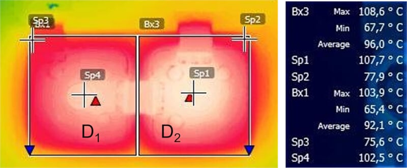
Figure 3. IR evaluation of a thermal measurement. Image used courtesy of Bodo’s Power Systems [PDF]

Comparing the Methods

A comparison of the three methods for averaging—in-situ, area average, and 2/3 approximation—results in slightly different numerical values. If the tolerances of the respective measuring techniques are considered, the values usually only deviate slightly from each other in the range of ±1 K.

Figure 3 gives insight into the data obtained using an IR camera from measuring two diodes connected in parallel within a semiconductor module.

The measuring points Sp₁ and Sp₄ in the middle of the diodes and Sp₂ and Sp₃ at their corners, clearly visible in Figure 3, are used for the 1/2 weighting. These measuring points were placed by hand, so there are also tolerances here. Based on the local values determined, the virtual chip temperatures for the diodes are:

\[T_{vj,D1}=\frac{1}{3}\cdot\Big(2\cdot T_{SP4}+T_{SP3}\Big)=\frac{1}{3}\cdot\Big(2\cdot102,5+75,6\Big)\degree C=93,5\degree C\]

\[T_{vj,D2}=\frac{1}{3}\cdot\Big(2\cdot T_{SP1}+T_{SP2}\Big)=\frac{1}{3}\cdot\Big(2\cdot107,7+77,9\Big)\degree C=97,8\degree C\]

The evaluation of the mean value over the entered areas Bx1 and Bx3 and the automatically displayed maxima and minima provide:

\[T_{vj,Bx1}=\frac{1}{3}\cdot\Big(2\cdot 103,9+65,4\Big)\degree C=91\degree C,\,\overline{T_{avg,com}}=92,1\degree C\]

\[T_{vj,Bx3}=\frac{1}{3}\cdot\Big(2\cdot 108,6+67,7\Big)\degree C=95\degree C,\,\overline{T_{avg,com}}=96\degree C\]

This means a temperature of 92.25±1.25°C for diode D1 and 96.4±1.4°C for diode D2. Although neither the true maximum nor the true minimum was met in both cases, the deviation of the values finally determined is negligible.

What is the practical use and gain for developers? Determining the chip temperature is crucial to support simulation results that are often starting points when predicting the lifetime of a system under development. Chiptemperature measurement during operation tends to be challenging. Thus, the recurring request is to get a customized power device with a thermal sensor attached to the chip. Instead—and if chip sizes allow—placing two sensors will get a very accurate result of the chip temperature, even under operating conditions. The similar results of all methods substantiate how robust the 1/2 averaging is when there is a setup with two thermocouples.

This article originally appeared in Bodo’s Power Systems [PDF] magazine.