Analytical Model of an LLC Converter with a Constant Power Load

The development of power conversion in the fields of electric vehicles, medical equipment, consumer goods, etc. combined with the need for high efficiency, has pushed the LLC architecture to the top. INFINERGIES, a power electronic design office, started thinking about new analytical models for this architecture.

In the domain of power electronics, the LLC converter is becoming more and more popular due to its interesting properties such as high boosting efficiency and low switching losses. But designing such a converter is quite challenging, and most of the time we need a mathematical model that generally uses a resistive load. This model has limitations and one of them is that loads, in general, aren’t only resistive at all times. In fact, the output voltage and current levels are variables depending on the needs. Most of the time the main output characteristic will be the power level because the load could be for example a point of load converter operating as a power load, as it maintains a constant output voltage for a constant-current load regardless of input voltage variation. In other applications, such as battery chargers, the control law of the converter can impose a behavior on the load, in which case it is preferable to deliver constant power to the battery in order to minimize its charging time. As a consequence, a model based on constant power loads seems more suitable when designing LLC converters.

 

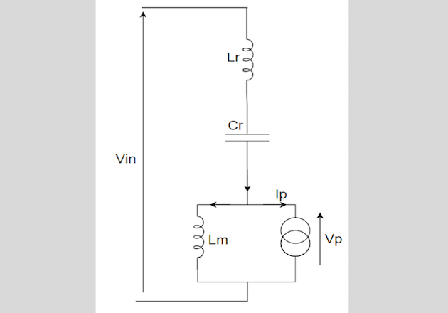
Figure 1: Primary-side model of the LLC converter

 

The Power Model

This model for the LLC converter is focused on the primary side. The rectifier and load on the secondary side are modeled as a primary side current source, whose current is output-voltage dependant. The power used by the current source is equivalent to the power used by the load. The first harmonic approximation is applied both to the input and output voltage. The resulting model is as shown in Figure 1.

The first harmonic approximation of the output voltage as seen on the primary side is:

 

$$V_p = \left ( \frac{4 \times n}{\pi} \right ) \times V_{out}$$

 

Where Vout is the output DC voltage, and n the transformer turns ratio Np/Ns. Since both the voltage and current are sine waves in first harmonic approximation, the output power Pout is:

 

$$P_{OUT} = V_{OUT} \times I_{OUT} = \frac{V_p \times I_p}{2}$$

 

Where Ip and Vp are in phase, the first harmonic approximation of the current is:
 

$$I_p - \frac{1}{n} \times \frac{\pi}{2} \times I_{OUT}$$

 

Likewise, for a full bridge LLC, the input voltage first harmonic approximation is:

 

$$V_{in} = \left ( \frac{4}{\pi} \right ) \times V_{dc}$$

 

Where Vdc is the input DC voltage. Vout and Iout both depend on the input voltage (Vin), the targeted output power level (Pout), the resonant inductor value (Lr), the resonant capacitor value (Cr), the magnetizing inductor value (Lm), the switching frequency (f) and the transformer turns ratio (n). The Vout curve represents the output voltage that the system should provide for fixed output power and at a defined switching frequency.

Model verification and limitations To verify our power model, we needed to compare results such as output voltage curves to ones from a common design which will be our benchmark. We went and used the common method seen is general application notes from semiconductor manufacturers using a resistive load and we calculated values for Lr, Cr, Lm and n using the following specifications given for a battery charger:

• Vin = 400V
• Vout = 250V - 500V
• Pout = 7kW
• Fres = 180kHz
• Fmin = 100kHz
• Fmax = 350kHz

The calculated component values to respect the above specifications are:

• Lr = 11 µH
• Cr = 73nF
• Lm = 21µH
• n = Np/Ns = 1
• Rout = 8.9Ω (7kW for Vout = 250V)
• Rout = 21Ω (7kW for Vout = 380V)
• Rout = 36Ω (7kW for Vout = 500V)

From the application notes data, we deduce a Vout expression (output voltage) for a fixed value of resistor which corresponds to only a single power level at a given frequency. Therefore, the output power level won’t be constant through a range of switching frequencies. In fact, it will vary according to the switching frequency. Pout is a function of the switching frequency:

 

$$P_{OUT}(f,R) = \frac{(V_{OUT}(f,R))^2}{R}$$

 

This varying output power will be used in our model to compare to the standard resistive load-based model. With such a varying power, our power load model should be equivalent to the resistive load model, which will allow for a comparison of the two models. Figure 2 shows the voltage versus frequency curve based on the resistive load model from the application notes (Vout_AN), and the voltage versus frequency curve based on the power load model (Vout_PM), with a power load varying based on the frequency as it would with the resistive model, such that the power used by the load in both models are identical at all frequencies.

 

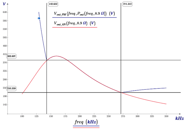
Figure 2: Output voltage of the LLC converter with a resistive load model, and with a constant power load model using a resistive load of 8.9Ω

 

As we can see, there is a significant frequency range (143kHz – 272kHz) where both curves are superposed. This demonstrates that our model is valid across this frequency range.

 

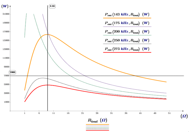
Figure 3: Power delivered by the LLC converter with a resistive load

 

From 143kHz to 272kHz, for Rout = 8.9Ω, both curves are completely identical. But below 143kHz and above 272kHz, they aren’t equivalent anymore. Figure 3 shows the output power of the LLC (resistive load mode) for fixed frequency values and Rout ranging from 1Ω to 50Ω.

We can see from this set of curves that, at the frequencies where both models stop matching, the power used by the load behaves differently for resistive values above and below the value used in Figure 2. For higher resistive values, the power used by the load decreases as the resistive value increases. The condition below, in this case, is respected:

 

$$\left ( \frac{V_{outAN} (freq,R)^2}{dR} |_r < 0 \right )$$

 

Additional verifications show that for any resistive load above this threshold value, the power load model and the resistive load model match at this frequency. We can generalize the principle as follows: the constant power model and the constant resistance model are consistent for any load and frequency where the following condition is respected:

 

$$\frac{d \left ( \frac{V_{outAN} (freq,R)^2}{R} \right )}{dR} < C$$

 

The reason for the mismatch between the two models is that there are two different resistive loads for every possible power level that can be reached by the converter. For a constant power load, only one of them is a stable equilibrium. The constant power model only matches the resistive model when the equivalent resistive load is the stable equilibrium setpoint.

It should be noted that simulation results match with the mathematical model, including in conditions where the two models diverge. Such a comparison is too long to be detailed in this article.

 

Model Results

Now that we have verified that the constant power load model is consistent with the literature, we can confidently predict the behavior of an LLC converter with such a load. Figures 4 shows a comparison of the output voltage of the LLC converter with a constant power load and a resistive load. The plot compares a resistive load model of 11Ω and a constant power load model of 7000 watts.

As we can see on these plots, there are two points of intersection between the two curves. The first one is at the resonant frequency which is always happening regardless of the power level because, for both models, the output voltage is independent of the load at the resonant frequency. The second one is at the frequency where the loads in both models are equivalent, here at 234kHz: at this frequency, the resistive model predicts a 7000 W output power for a 11Ω load resistance, and therefore it intersects with the 7000W constant power model curve (see Figure 4).

 

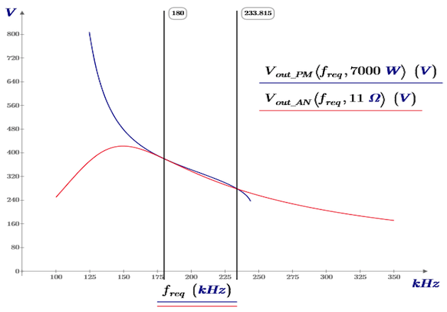
Figure 4: Output voltage of the LLC converter with a resistive load and a constant power load

 

Figure 4 reveals two significant differences between the two models. The first difference is that there is a limit to the power that can be delivered by the converter at a given frequency, and this maximum power decreases as the frequency increases from a threshold value. The equation of the output voltage as a function of frequency and power doesn’t have any real solution above a certain frequency. This means that it is impossible for this converter to deliver 7kW for frequencies above 243kHz. Figure 5 shows that lower power levels can be reached at frequencies higher than 243kHz.

 

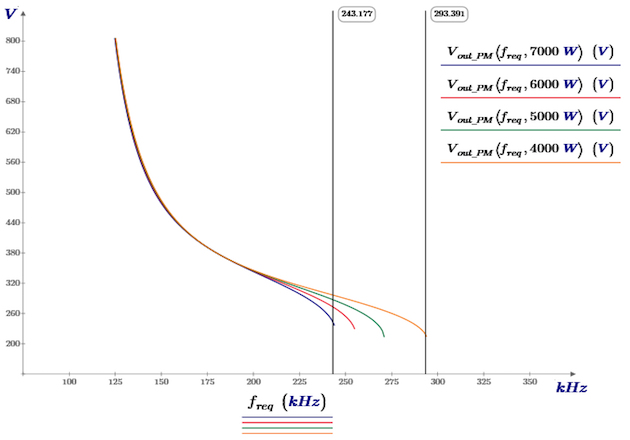
Figure 5: Output voltage of the LLC converter with a constant power load

 

The second significant difference is that there is no limit to the maximum output voltage. The model diverges (Vout → ∞) at the secondary resonant frequency;

 

$$F_{R_2} = \frac{1}{2 \times \pi \times \sqrt{(L_r + L_m) \times C_r}}$$

 

Unlike with a resistive load, an LLC converter with a constant-power load can reach very high voltages. This can be very useful in some applications, such as battery chargers because the maximum output voltage that needs to be reached is no longer a major constraint on the design. It can also be dangerous for the load or the converter, in case of control loop failure that would set the switching frequency to the minimum frequency. Independent protections should be implemented to avoid such damages.

We should note that the phasing of the resonant current wasn’t considered in this study. Although it is possible to reach high voltages at low frequency, it may or may not be possible to achieve zero voltage switching when doing so.

 

A Difficult Topology to Model

The resistive load model described in most application notes has many advantages, such as the normalization of the design parameters. However, it is not representative of many types of loads (POL converters, batteries…), and a new, updated model is required for a better design. First, the constant power load model shows value-added information on the LLC design. And secondly, it speeds up the design for all constant power loads.

However, some loads may have yet another kind of behavior. Some loads, such as deeply discharged batteries, can require a constant current source. Another model is then required for the converter. We will present such a model in a future article.

 

About the Authors

Oumar Thiam is an engineer at INFINERGIES, a company that specialized digitally controlled power electronics with services such as custom power converters design, design of mock-ups and proofs-of-concept, and other high value-added power electronics related service.

Adrien Thurin received his master's degree in power electronics, electrotechnics, and control at CentraleSupélec  French graduate school of engineering. He is the CEO and co-founder of INFINERGIES, a company that specialized digitally controlled power electronics with services such as custom power converters design, design of mock-ups and proofs-of-concept, and other high value-added power electronics related service.

Julien Ménagé has an engineering degree at CentraleSupélec and works as a general manager for INFINERGIES, a company that specialized digitally controlled power electronics with services such as custom power converters design, design of mock-ups and proofs-of-concept, and other high value-added power electronics related service.

 

This article originally appeared in the Bodo’s Power Systems magazine.