Facebook
 Google
 GitHub
 Linkedin
An Introduction to the Fall-of-Potential Method
Learn about the fall-of-potential method of determining the resistance of a grounding electrode.
There are several methods and formulas to calculate the resistance to earth of the grounding electrode system during the design phase. All these methods and formulas have an error margin, and the soil resistivity — a constant in all formulas — is neither constant nor uniform. The earth resistivity of the area where the grounding electrode system will be embedded must be quantified in the design phase, and the resistance to earth tested after the construction. The Fall-of-Potential Method is the most used approach for measuring resistance to earth.
The Fall-of-Potential Method
The fall of potential method accurately tests the resistance of a grounding electrode.
The basis of this method is Ohm’s law. Ohm's law states that applying a potential difference between two points causes a flow of charge, and the opposition to this flow is the resistance encountered. Then,
Current = potential difference/resistance, or, I(amperes) = V(volts)/R(ohms)
Ohm’s law led to our concept of resistance and the unit of an ohm for measuring it. If we apply a potential difference to any conductor and measure the current that results, the resistance of the conductor is the voltage drop divided by the current.
That is,
R(ohms) = V(volts)/I(amperes).
This equation is the definition of electrical resistance.
Ohm’s law considers a constant resistance. In our case, the resistance is not constant, as can be deduced from Figure 1. Then, we’ll use a graphical method to ascertain the electrode’s resistance.
The fall-of-potential method consists (shown in Figure 1) of circulating AC or DC current between the electrode under test (electrode 1) and a fixed electrode (electrode 2), and measuring the voltage drop between electrode 1 and a movable electrode (electrode 3).
Now there are three electrodes with infinite layers wrapping around them. Commercial measuring equipment does not use hemispheric electrodes but simple ground rods. The behavior of the earth resistance, however, is in harmony with that studied for hemispheric electrodes.
To measure the current through the circuit, we cause it to flow through an ammeter. To measure the voltage drop, we connect a voltmeter, as shown. The ammeter has low resistance and the voltmeter high resistance, with minimum impact on the measurement results.
The ratio of the measured voltage drop to the circulating current gives the resistance value at the position of electrode 3.
The earth testing equipment does the calculations internally and displays the amount of resistance directly in ohms. Occasionally, transmission and distribution applications, where distance D can be enormous, require specialized techniques and instrumentation.
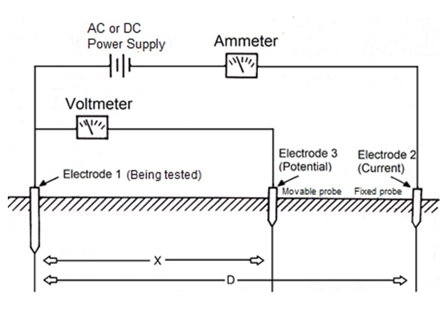
Figure 1. Fall-of-potential test set-up. Image-based on a drawing from Megger.
The resistance quantities will vary, as recorded in table 2 and displayed in Figure 3 when moving the electrode 3 along a straight line between electrodes 1 and 2.
Table 1 Per-unit resistance quantities of a grounding electrode and test probe
| n (1) |
R (P.U.) (2) |
Incremental R(P.U.) (3) |
na (4) |
Cumulative ground R (P.U.) (5) |
% of total R (6) |
% of total na = %D (7) |
| 1 | 0.000 | 0.000 | 1 | 0.000 | 0.0 | 0.5 |
| 2 | 0.500 | 0.500 | 2 | 0.500 | 25.3 | 1.0 |
| 5 | 0.800 | 0.300 | 5 | 0.800 | 40.4 | 2.5 |
| 10 | 0.900 | 0.100 | 10 | 0.900 | 45.5 | 5.0 |
| 15 | 0.933 | 0.033 | 15 | 0.933 | 47.1 | 7.5 |
| 20 | 0.950 | 0.017 | 20 | 0.950 | 48.0 | 10.1 |
| 25 | 0.960 | 0.010 | 25 | 0.960 | 48.5 | 12.6 |
| 30 | 0.967 | 0.007 | 30 | 0.967 | 48.8 | 15.1 |
| 35 | 0.971 | 0.005 | 35 | 0.971 | 49.1 | 17.6 |
| 40 | 0.975 | 0.004 | 40 | 0.975 | 49.2 | 20.1 |
| 45 | 0.978 | 0.003 | 45 | 0.978 | 49.4 | 22.6 |
| 50 | 0.980 | 0.002 | 50 | 0.980 | 49.5 | 25.1 |
| 55 | 0.982 | 0.002 | 55 | 0.982 | 49.6 | 27.6 |
| 60 | 0.983 | 0.002 | 60 | 0.983 | 49.7 | 30.2 |
| 65 | 0.985 | 0.001 | 65 | 0.985 | 49.7 | 32.7 |
| 70 | 0.986 | 0.001 | 70 | 0.986 | 49.8 | 35.2 |
| 75 | 0.987 | 0.001 | 75 | 0.987 | 49.8 | 37.7 |
| 80 | 0.988 | 0.001 | 80 | 0.988 | 49.9 | 40.2 |
| 85 | 0.988 | 0.001 | 85 | 0.988 | 49.9 | 42.7 |
| 90 | 0.989 | 0.001 | 90 | 0.989 | 49.9 | 45.2 |
| 95 | 0.989 | 0.001 | 95 | 0.989 | 49.9 | 47.7 |
| 100 | 0.990 | 0.001 | 100 | 0.990 | 50.0 | 50.3 |
| 95 | 0.989 | 0.001 | 105 | 0.991 | 50.0 | 52.8 |
| 90 | 0.989 | 0.001 | 110 | 0.991 | 50.1 | 55.3 |
| 85 | 0.988 | 0.001 | 115 | 0.992 | 50.1 | 57.8 |
| 80 | 0.988 | 0.001 | 120 | 0.993 | 50.1 | 60.3 |
| 75 | 0.987 | 0.001 | 125 | 0.993 | 50.2 | 62.8 |
| 70 | 0.986 | 0.001 | 130 | 0.994 | 50.2 | 65.3 |
| 65 | 0.985 | 0.001 | 135 | 0.995 | 50.3 | 67.8 |
| 60 | 0.983 | 0.001 | 140 | 0.997 | 50.3 | 70.4 |
| 55 | 09.82 | 0.002 | 145 | 0.998 | 50.4 | 72.9 |
| 50 | 0.980 | 0.002 | 150 | 1.000 | 50.5 | 75.4 |
| 45 | 0.978 | 0.002 | 155 | 1.002 | 50.6 | 77.9 |
| 40 | 0.975 | 0.003 | 160 | 1.005 | 50.8 | 80.4 |
| 35 | 0.971 | 0.004 | 165 | 1.009 | 50.9 | 82.9 |
| 30 | 0.967 | 0.005 | 170 | 1.013 | 51.2 | 85.4 |
| 25 | 0.60 | 0.007 | 175 | 1.020 | 51.5 | 87.9 |
| 20 | 0.950 | 0.010 | 180 | 1.030 | 52.0 | 90.5 |
| 15 | 0.933 | 0.017 | 185 | 1.047 | 52.9 | 93.0 |
| 10 | 0.900 | 0.033 | 190 | 1.080 | 54.5 | 95.5 |
| 5 | 0.800 | 0.100 | 195 | 1.180 | 59.6 | 98.0 |
| 2 | 0.500 | 0.300 | 198 | 1.480 | 74.7 | 99.5 |
| 1 | 0.000 | 0.500 | 199 | 1.980 | 100.0 | 100.0 |
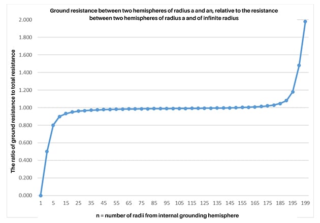
Figure 2. A plot of per-unit resistance of a grounding electrode and test probe.
Table 1 and Figure 2 show an outcome when the layers of electrodes 1 and 2 interfere (overlap) each other. As we progress from electrode 1 in a straight line toward electrode 2, the ground resistance rises quickly in the first few layers and then flattens out. At one point, the curve picks up the layers of electrode 2, and the resistance continues to increase, slowly at the beginning and rapidly at the end. The almost horizontal section in the middle portion of the curve is the earth resistance.
When the distance D between electrodes 1 and 2 is enormous, the resistance values measured are more accurate because there is little interference between the electrode layers.
The approximate value of the earth resistance is the ratio of the voltage drop and current when the separation X, between electrodes 1 and 3, is about 62% of the distance D (X = 0.62 D).
Table 2 and Figure 3 show a relatively constant (flat) resistance zone between 52.8% and 62.8% of distance D, with a resistance range from 0.991 P.U. to 0.993 P.U.
The curve, when plotted on-site, displays the ohm readings provided by the earth testing equipment. Then, the resistance read in the flat area of the curve, roughly at 62% of D, is the approximate earth resistance.
Stray currents can greatly distort the results. But modern measuring equipment can reduce errors.
The Effect of Placing Electrodes 1 and 2 Exceedingly Close
If electrode 2 is close to electrode 1, their layers interfere with each other, and the resistance curve results in the way shown in Table 2 and Figure 3.
Table 2 Per-unit resistance quantities of a grounding electrode and test probe, closely spaced
| n (1) |
R (P.U) (2) |
Incremental R (P.U.) (3) |
na (4) |
Cumulative ground R (P.U.) (5) |
% of total R (6) |
% of total na = %D (7) |
| 1 | 0.000 | 0.000 | 1 | 0.000 | 0.0 | 2.6 |
| 2 | 0.500 | 0.500 | 2 | 0.500 | 26.3 | 5.1 |
| 5 | 0.800 | 0.300 | 5 | 0.800 | 42.1 | 12.8 |
| 10 | 0.900 | 0.100 | 10 | 0.900 | 47.4 | 25.6 |
| 15 | 0.933 | 0.033 | 15 | 0.933 | 49.1 | 38.5 |
| 20 | 0.950 | 0.017 | 20 | 0.950 | 50.0 | 51.3 |
| 15 | 0.933 | 0.017 | 25 | 0.967 | 50.9 | 64.1 |
| 10 | 0.900 | 0.033 | 30 | 1.000 | 52.6 | 76.9 |
| 5 | 0.800 | 0.100 | 35 | 1.100 | 57.9 | 89.7 |
| 2 | 0.500 | 0.300 | 38 | 1.400 | 73.7 | 97.4 |
| 1 | 0.000 | 0.500 | 39 | 1.900 | 100.0 | 100.0 |

Figure 3. A plot of per-unit resistance of a grounding electrode and test probe, closely spaced
The resistance curve has a point of inflection where it changes from concave down to concave up, but it always increases and does not exhibit the flat area that allows us to deduce the approximate earth resistance.
A rule of thumb used to determine the minimum electrode spacing (D) is to calculate the most significant length of the grounding electrode and multiply by 10. For example, if the grounding electrode is a single 3 m long rod, the minimum spacing is 30 m. For a rectangular ground mat, find the length of the diagonal and multiply by 10. Note that for a large mat, the separation D could be on the order of kilometers, and the application of this method would require special techniques and instrumentation.
A practical procedure is to make the first measurement by placing electrode 3 at 0.5·D and then moving it to both sides, making two or three additional measurements in each direction. If the results indicate that you are in the flat area, the value of the resistance to earth is the average of the measurements. Otherwise, increase D and try again.
As a last resort, if the available space does not allow adequate separation, take the resistance value at the inflection point. This number will not be the best, but there is no other option.
In the next article of this series, we will look at the pros and cons of the fall-of-potential method, as well as other methods for testing the earth’s resistance to grounding electrodes.