Facebook
 Google
 GitHub
 Linkedin
The Earth Resistance of a Grounding Electrode
Learn about the make-up of the resistance of a grounding electrode to infinity.
One of the distinctive parameters of the grounding electrodes is the resistance to earth. This number is an indicator, although not final, of the proper functioning of the grounding system. A grounding electrode radiates current in all directions, so it is surrounded by many layers, each with a certain amount of resistance. The total resistance to earth is the sum of the resistances of all these layers to infinity.
The resistance to earth of an electrode consists of three components: metal resistance, contact resistance, and resistance to the flow of current through the soil.
The material of grounding electrodes is a very conductive metal with a suitable cross-section, so their resistance is not significant. The contact resistance between the electrode and the compacted earth around it, being free of paints, oils, or other coatings, is also negligible. The resistance of the ground touching the electrode, up to infinity, is significant and will be the subject of the analysis below.
Imagine the grounding electrode inserted into the center of a big onion, and you measure the resistance from the electrode to the surface of the onion. The onion consists of many concentric layers, and we can assume that each of these layers has a resistance value. If we measure the resistance of each one and add them up, we will obtain the total resistance.
The earth is not an onion, but this simile will help you better understand how the total resistance of the electrode to infinity, comes from the sum of many resistances in series, one per layer.
The following four factors determine the resistance of a wire with a uniform cross-sectional area:
- Kind of material
- Cross-sectional area
- Length
- Temperature
The resistance of a conductor at 20°C is R = ρ · L/A, where:
ρ = resistivity of the material (ohm·cm or ohm·m)
L = length (cm or m)
A = cross-sectional area (cm² or m²)
Although this equation involves metals, it also applies satisfactorily to most non-metallic conductors such as the earth.
The resistance equation shows that it is directly proportional to the length and resistivity of the conductor and inversely proportional to the cross-sectional area. The higher the length or resistivity, or the smaller the area, the higher the resistance.
Let’s calculate the resistance of a hemispheric grounding electrode of radius a as a function of the distance to an imaginary outer hemispheric electrode of radius r.
The surface area of a sphere is A = 4·π·r² where r is the radius of the sphere. The area of half a sphere, or hemisphere, is A = 2·π·r².
At this point, we can infer that as we move away from the electrode, the hemispheric layers will have larger areas, and therefore, their resistance will be lower. Then, as we add resistances in series, the result will increase rapidly with the nearer hemispheric layers and slowly as we move away towards infinity. This conjecture will be demonstrated mathematically in the following paragraphs.
The most suitable mathematical tool to add up these infinite number of resistances is integral calculus.
The differential resistance dR between two hemispheric layers separated by a distance dr is:
dR = (ρ/2·π) · 1/r² · dr
Integrating between the radius a of the electrode and a layer at a distance r,
$$\int ^r_a dr = \frac{1}{a} = \frac{1}{r}$$
Then,
R = (ρ/2·π) · (1/a – 1/r) Ω where,
a = radius of hemispherical electrode
r = radius of outside hemisphere
Defining r = na, where n = 1, 2, 3,…,∞
R = (ρ/2·π) · (1/a – 1/na) Ω
R = (ρ/2·π· a) (1 - 1/n) Ω Equation 1
Two boundary values of resistance are n = 1, and n = ∞.
For n = 1, R = 0 Ω, and for n = ∞, R = ρ/2·π· a Ω.
These boundary values mean that the resistance starts with zero ohms at the surface of the hemispheric electrode and reaches ρ/2·π· a ohms at infinity. Between these two extreme values, there is an endless collection of resistance values. The total resistance increases as we move away from the hemispheric electrode but at a decreasing rate.
Table 1 shows per-unit (P.U.) resistance quantities for selected values of n. The base of the per-unit figures is the resistance at infinity, i.e., R = ρ/2·π·a.
Table 1 Per-unit resistance quantities of a hemispheric ground electrode
| n (1) |
R (P.U.) (2) |
Incremental R (P.U.) (3) |
na (4) |
Cumulative |
% of total R (6) |
% of total na = %D (7) |
| 1 | 0.000 | 0.000 | 1 | 0.000 | 0.0 | 1.0 |
| 2 | 0.500 | 0.500 | 2 | 0.500 | 50.0 | 2.0 |
| 5 | 0.800 | 0.300 | 5 | 0.800 | 80.0 | 5.0 |
| 10 | 0.900 | 0.100 | 10 | 0.900 | 90.0 | 10.0 |
| 15 | 0.933 | 0.033 | 15 | 0.933 | 93.3 | 15.0 |
| 20 | 0.950 | 0.017 | 20 | 0.950 | 95.0 | 20.0 |
| 25 | 0.960 | 0.010 | 25 | 0.960 | 96.0 | 25.0 |
| 30 | 0.967 | 0.007 | 30 | 0.967 | 96.7 | 30.0 |
| 35 | 0.971 | 0.005 | 35 | 0.971 | 97.1 | 35.0 |
| 40 | 0.975 | 0.004 | 40 | 0.975 | 97.5 | 40.0 |
| 45 | 0.975 | 0.003 | 45 | 0.978 | 97.8 | 45.0 |
| 50 | 0.980 | 0.002 | 50 | 0.980 | 98.0 | 50.0 |
| 55 | 0.982 | 0.002 | 55 | 0.982 | 98.2 | 55.0 |
| 60 | 0.983 | 0.002 | 60 | 0.983 | 98.3 | 60.0 |
| 65 | 0.985 | 0.001 | 65 | 0.985 | 98.5 | 65.0 |
| 70 | 0.986 | 0.001 | 70 | 0.986 | 98.6 | 70.0 |
| 75 | 0.987 | 0.001 | 75 | 0.987 | 98.7 | 75.0 |
| 80 | 0.988 | 0.001 | 80 | 0.988 | 98.8 | 80.0 |
| 85 | 0.988 | 0.001 | 85 | 0.988 | 98.8 | 85.0 |
| 90 | 0.989 | 0.001 | 90 | 0.989 | 98.9 | 90.0 |
| 95 | 0.989 | 0.001 | 95 | 0.989 | 98.9 | 95.0 |
| 100 | 0.990 | 0.001 | 100 | 0.990 | 99.0 | 100.0 |
The columns in Table 1 ask for a detailed explanation.
Column 1, n, is the number of radii from the hemispherical electrode.
Column 2, R (P.U.), is the per-unit resistance at a distance na computed with equation 1 and normalized to the base quantity.
Column 3, incremental R (P.U.), is row n minus row (n-1) in column 2. It is the resistance increase in this step.
Column 4, na, is the actual distance in meters, centimeters, or any chosen unit, from the hemispherical electrode. In this example a = 1, then na = n.
Column 5, cumulative ground R, is the sum of row n plus row (n-1) in column 3. In this example, there is no interference from another electrode, then column 5 = column 2.
Column 6, % of total R, is the P.U. value times 100. Note that 100% of R is reached only at infinity.
Column 7, % of total na = %D, is the distance as percentage of the maximum length in the example (D).
Figure 1 uses columns 1 and 2 to show the rise of the resistance (P.U.) graphically as the distance increases. Figure 1 is a well-known plot in grounding analysis and design.
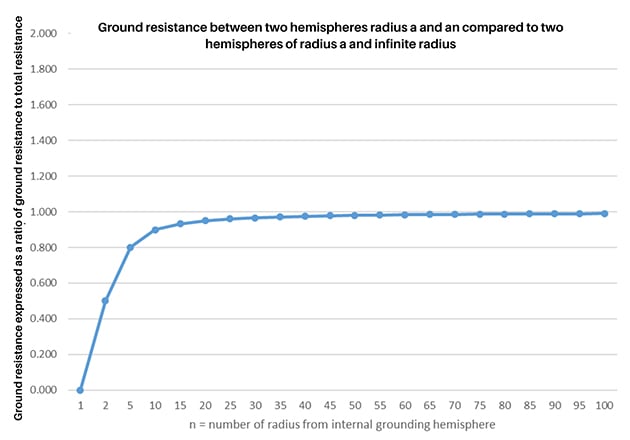
Fig. 1 This plot illustrates changes in ground resistance relative to the distance from the electrode. Resistance increases rapidly near the electrode, and at larger distances, it asymptotically approaches the total resistance.
These results lead to the following conclusions:
- The highest percentage of the total resistance emerges in the layers closest to the grounding electrode. n = 10 achieves 90% of the total resistance.
- The resistance curve is asymptotic to 1 P.U.
In the second article of this series, we will analyze the fall-of-potential method.