Facebook
 Google
 GitHub
 Linkedin
What Are Magnetically Coupled Inductors?
This article discusses magnetically coupled inductors, more commonly known as transformers.
This is just one of a number of articles in the EE Power inductor series. Please see the rest of the articles here:
A transformer is a passive AC circuit device that performs a voltage transformation to either step up or step down the input voltage.
The Basic Transformer Equation
Faraday’s law for a single conductive loop is:
\(\varepsilon=-\frac{d\phi}{dt},\) [1]
where ε is the electromotive force, or voltage, and dΦ/dt is the rate of change of magnetic flux with time.
A multi-turn coil is the equivalent of individual loops connected in series, therefore the voltages add and Faraday’s law becomes:
\(\varepsilon=-\frac{Nd\phi}{dt},\) [2]
For two separate coils wound around the same magnetic core with perfect flux coupling, the dΦ/dt is common, so
\(\varepsilon_{1}=-\frac{N_{1}d\phi}{dt},and\)
\(\varepsilon_{2}=-\frac{N_{2}d\phi}{dt},therefore\)
\[\frac{\varepsilon_{1}}{\varepsilon_{2}}=\frac{N_{1}}{N_{2}},\]
which says the voltage ratio equals the turns ratio and this is the fundamental defining equation of transformer operation.
Field Strength and Frequency
Rewriting Equation [1] in integral form gives:
\(\Phi=-\int\varepsilon dt\) [3]
If the applied voltage is sinusoidally time varying, then Equation [3] can be written as
\[\Phi=-\int\varepsilon_{0}sin(\omega t)dt\]
\[=\frac{\varepsilon_{0}}{\omega}cos(\omega t)\]
This says that the flux is inversely proportional to the frequency of the applied voltage. Flux is the integral of the normal component of the magnetic field B over the cross-section of interest.
\[\Phi=\int Bd\,A\]
If Φ is sinusoidally time varying with an amplitude that is inversely proportional to frequency, then B must also be sinusoidally time varying with an amplitude inversely proportional to frequency and can be written as:
\(B=\frac{B_{0}}{\omega}cos(\omega t)\) [4]
The significance is that as the frequency of operation is decreased, the magnetic field strength increases.
The B-H Loop
In a ferromagnetic material, the total magnetic field in the material is the sum of the applied field and the internal field generated by the alignment of magnetic domains. The total field in the material is represented as B and over some linear region can be approximated as
\[B=\mu_{o}\mu_{r}H,\]
Where μo is the magnetic permeability of free space and μr is the relative permeability of the material, assuming a linear magnetic behavior. A representative B-H loop, which plots the field B as the applied field is cycled, is shown in Figure 1. At high magnetic field strengths the curve becomes very non-linear and the material is said to have reached magnetic saturation. As magnetic saturation is approached, an increase in H results in a much lower increase in the value of B.
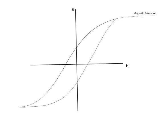
Figure 1. Representative B-H loop for a ferromagnetic material. Image used courtesy of Blaine Geddes
The energy dissipated in cyclically magnetizing the material is the hysteresis loss and is given as the integral of the B-H loop. The area of the B-H loop depends on the magnetic remanence of the material which is a function of the energy required to realign the domains. Ferromagnetic materials with low remanence are known as soft. Hard ferromagnetic materials have a much more open B-H loop because they tend to retain their magnetic state once magnetized. For use in AC circuits, clearly soft ferromagnetic materials are much preferred.
As magnetic saturation is reached, not only is the hysteresis loss at a maximum, but any increase in current flow produces a negligible increase in the magnetic field strength, so it is just wasted as I2R losses in the windings.
From Equation [4], the magnetic field rises as the applied frequency is reduced, so to avoid magnetic saturation, the physical size of AC magnetic devices such as transformers, motors, etc., must be made larger as the line frequency is lowered.
Sizing the Core
The maximum working field strength for silicon electrical steel is typically in the 1.3 – 1.7 T range, although some grain-oriented alloy steels can support higher field strengths. The saturation field strength of M-6 electrical steel (grain oriented 3% Si) is specified as 1.9 T. The closer to magnetic saturation that the core is required to operate, the greater the losses, so some margin is required. The first step in sizing the core will be to choose the allowable maximum operating magnetic field strength in the core, and this will be dependent on the grade of electrical steel chosen for the core.
Faraday’s law for a multiturn coil gives dΦ/dt for a given applied voltage and number of turns. Integrating dΦ/dt will give the total flux Φ. For a sinusoidal circuit, Φ will be sinusoidal with a 1/ω factor on its amplitude.
Applying = BdA, allows the field B to be determined for a given core area, or the area to be determined given a specified maximum allowable field B. Increasing the cross-sectional area or increasing the number of turns will reduce the maximum field strength, so these are the main variables of adjustment to provide an acceptable design respecting size, cost, and performance trade-offs. Transformer size scales inversely with frequency, so the line frequency is a vital parameter. A transformer designed for 60 Hz, will work acceptably at 120 Hz, although it will be oversized, but it may become very inefficient and overheat if operated at 30 Hz.
Once the number of turns is chosen for the primary winding based on the above considerations of trading off the number of turns and core cross-sectional area to achieve an acceptable maximum field strength B, the number of turns in the secondary winding is simply set by the desired voltage ratio. The core also needs enough space to accommodate the winding coils. The wire gauge of the coils will be set by the required current flow to keep the current density in the windings at an acceptable level to minimize I2R losses in the windings. The core window area must be large enough to accommodate the windings which scales with the number of turns and the required wire gauge based on maximum current flow.
Applying all of the equations and the tradeoffs makes transformer design an iterative procedure where some assumptions would need to be made and calculations repeated. Various formulas have been developed for estimating a core size given the inputs of Volt-Ampere rating for the transformer, maximum allowable B field, lowest operating frequency, core geometry parameters, and possibly other parameters such as wire resistivity, allowable conductor losses, etc. All such formulas are based on the fundamental principle of Faraday's law and basic geometry.
A transformer is a deceptively simple passive device, but designing one involves manipulating many variables to produce a properly optimized design.
Transformer Construction
Transformers for power line frequencies and frequencies up to a few kilohertz are constructed of interleaved sheets of electrical steel stamped to shape to provide the core for the coil and a window area for the windings. The laminated structure reduces eddy current losses. The surfaces of the sheets are coated with a thin layer of a high resistivity finish. Figure 2 shows a typical transformer indicating its laminated core structure. Various core geometries are common. This one has its windings wound together in the same form.
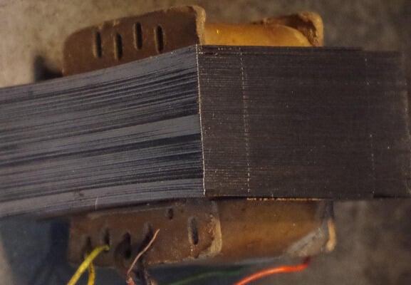
Figure 2. Photograph of a transformer showing the laminated core structure. The dotted seam indicates how the sheets are interleaved. Image used courtesy of Blaine Geddes
Transformer Equivalent Circuit
An equivalent circuit of a transformer with all quantities referred to the primary side is shown in Figure 3. The quantities from the secondary side reflect to the primary with a 1/N2 factor, where N is the secondary to primary turns ratio.
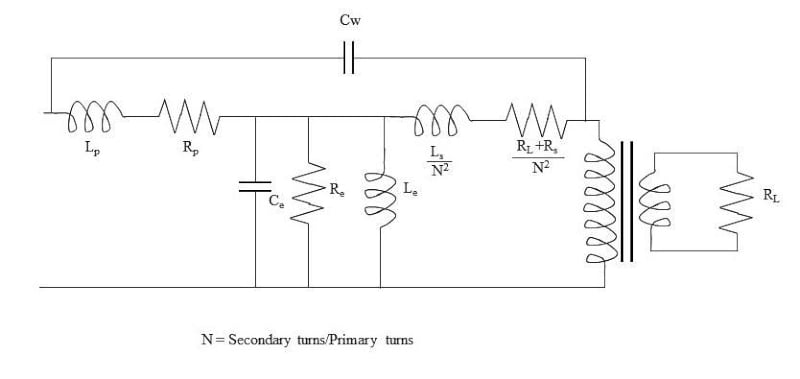
Figure 3. Equivalent circuit of a transformer with all quantities referred to the primary side. Image used courtesy of Blaine Geddes
In the equivalent circuit model, RL is the load resistance. Rs is the secondary winding resistance. Ls is the secondary winding inductance. Rp and Lp are the primary winding resistance and inductance, respectively. Re represents the core losses and it is composed of eddy current losses and hysteresis losses. Le represents the effect of cyclical magnetization of the core, which involves the shifting of domains of the ferromagnetic material, so it is modeled as an inductor.
The parasitic capacitances created by the close interwinding spacings and the windings to case capacitance are lumped together as a single pair of capacitors, Cw and Ce, but they are complicated because of the many windings creating a myriad of parasitic capacitance effects. Fortunately, these capacitive effects are small and can be neglected at low frequencies.
Transformers at High Frequencies
The physical size of inductors and transformers shrinks as the frequency of operation increases because of the 1/ω effect on the flux density in the core.
Hysteresis losses increase with frequency because of the increased rate of cycling around the B-H loop, therefore, very soft ferromagnetic materials are required for high frequencies. Eddy current losses are proportional to the square of the frequency, because, by Faraday’s law, the induced voltage driving the eddy currents is proportional to dΦ/dt.
Laminated electrical steel core transformers are used to frequencies up to a few kiloHertz. For frequencies beyond about 10 kHz, ferrites are commonly used. Ferrites are ceramics. They are blends of metal oxides composed mainly of oxides of iron, manganese, zinc, and nickel. Ferrites have much lower permeabilities but vastly higher resistivities. The magnitude of the induced eddy current varies inversely with the material's resistance, so the eddy current I2R loss will drop proportionally with an increase in resistivity.
Featured image used courtesy of Adobe Stock