Tuned Coupled Coils Explained

Mutual inductance exists between adjacent coils, and when a current flows in one coil, a terminal voltage may be induced in a mutually coupled coil.

 

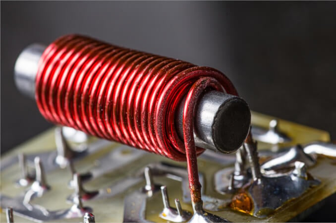
Image used courtesy of Adobe Stock

 

Figure 1(a) shows a typical arrangement of two mutually coupled coils wound on a nonmagnetic core. The coupling coefficient between the coils can be adjusted simply by altering the spacing between them. The circuit diagram for coupled coils is shown in Figure 1(b). Note the dots at one end of each coil. These are employed to show the phase relationship between input and output voltages. The dots simply identify the in-phase ends of each coil. Thus, when an input voltage applied to the left-hand coil has the instantaneous polarity shown (positive at the dotted end), the output voltage from the secondary (right-hand) coil is also positive at the dotted end of the coil.

 

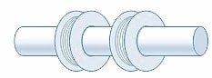
(a) Coupled coils.

 

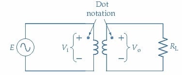
(b) Circuit diagram for coupled coils.

Figure 1. Coupled coils and their circuit diagram. The dot notation on the circuit diagram denotes the relative polarity of the coil input and output voltages. Image used courtesy of Amna Ahmad

 

The equivalent circuit for the coupled coils is shown in Figure 2. Resistor R₁ represents the resistive component of the primary winding, and L₁ is the inductive component. R₂ and L₂ are the total resistive and inductive components in the secondary winding, respectively. When a current (I₁) flows in the primary winding, a voltage \(\big(\omega MI_{1},\big)\) is induced in the secondary winding, causing a secondary current (I₂) to flow. The flow of I₂ also induces a voltage \(\big(\omega MI_{2},\big)\) in the primary winding. This induced voltage must be shown as having a polarity that opposes the primary current. The equivalent circuit includes two voltage generator symbols to represent the voltages induced in each winding.

 

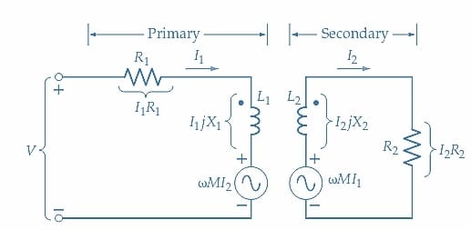
Figure 2. Equivalent circuit for coupled coils. Each coil has resistive and inductive components (R and L), and each has a voltage \(\big(\omega MI\big)\) induced by the current flow in the other coil. Image used courtesy of Amna Ahmad

 

Coupled Impedance

The equation for the voltage drops around the primary circuit may be written as

\[V=I_{1}R_{1}+jI_{1}X_{1}+\omega MI_{2}(1)\]

and the equation for the voltage drops around the secondary circuit is

\[\omega MI_{1}=I_{2}R_{2}+jI_{2}X_{2}\]

Which gives

\[I_{2}=\frac{\omega MI_{1}}{R_{2}+jX_{2}}(2)\]

Substituting for I₂ in Equation 1

\[V=I_{1}R_{1}+jI_{1}X_{1}+\frac{(\omega M)^{2}I_{1}}{R^{2}+jX_{2}}\]

The primary impedance is

\[Z_{1}=\frac{V}{I_{1}}\]

So

\[Z_{1}=R_{1}+jX_{1}+\frac{(\omega M)^{2}}{R_{2}+jX_{2}}(3)\]

The primary circuit impedance is seen to consist of a self-impedance Z and a coupled impedance Z₂ (coupled from the secondary into the primary), where the self-impedance is

\[Z=R_{1}+jX_{1}\]

The coupled impedance is

\[Z^{{\,}'}_{2}=\frac{(\omega M)^{2}}{R_{2}+jX_{2}}(4)\]

The coupled impedance can be resolved into resistive and reactive components by multiplying it by the conjugate of the denominator.

\[Z^{{\,}'}_{2}=\frac{(\omega M)^{2}}{R_{2}+jX_{2}}\times\frac{R_{2}-jX_{2}}{R_{2}-jX_{2}}\] 

\[=\frac{(\omega M)^{2}R^{2}-j(\omega M)^{2}X_{2}}{R^{2}_{2}+X^{2}_{2}}\]

\[Z^{{\,}'}_{2}=\frac{(\omega M)^{2}R_{2}}{R^{2}_{2}+X^{2}_{2}}-j\frac{(\omega M)^{2}X_{2}}{R^{2}_{2}+X^{2}_{2}}(5)\]

The coupled impedance is comprised of a coupled resistance \(R^{{\,}'}_{2} \) and a coupled reactance \(X^{{\,}'}_{2}\).

Coupled resistance is

\[R^{{\,}'}_{2}=\frac{(\omega M)^{2}R_{2}}{R^{2}_{2}+X^{2}_{2}}(6)\]

Coupled reactance is

\[X^{{\,}'}_{2}=-j\frac{(\omega M)^{2}R_{2}}{R^{2}_{2}+X^{2}_{2}}(7)\]

 

Coefficient of Coupling

Now consider the coupled circuits shown in Figure 3(a), in which the primary and secondary circuits include capacitors. The circuits are tuned to resonate at the same frequency, so the series reactance in each circuit is zero at the resonance frequency. When X₂ is zero, only the resistive component of the impedance is coupled from the secondary into the primary. Also, because of the presence of X₂ in the denominator of the expression for the coupled resistance (Equation 6), the coupled resistance is a maximum when X₂ becomes zero (i.e., at the resonance frequency). This (maximum) coupled resistance adds to the coil resistance of the primary and thus reduces the primary current at resonance.

 

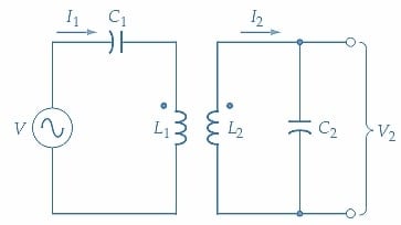
(a) Coupled coils tuned to resonate.

 

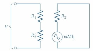
(b) The equivalent circuit at resonance

Figure 3. Coupled coils can be tuned to resonate at the same frequency by including appropriate capacitors in the primary and secondary circuits. At resonance, X_C1 and X_C2 cancel X_L1 and X_L2, respectively, and maximum primary and secondary currents flow. Image used courtesy of Amna Ahmad

 

Figure 3(b) shows the equivalent circuit of the coupled circuits at resonance. R₁ and R₂ are the primary and secondary coil resistances, respectively, and \(R^{{\,}'}_{2}\) is the secondary resistance coupled into the primary. At resonance (with X₂=0), Equation 6 for \(R^{{\,}'}_{2}\) becomes

\[R^{{\,}'}_{2}=\frac{(\omega M)^{2}}{R_{2}}(8)\]

Viewed from the input terminals, the primary circuit (operating alone) is a series resonant circuit with a maximum impedance at resonance

\[Z=R_{1}\]

The secondary circuit behaves as a series resonant circuit with a supply voltage of \(\big(\omega MI_{1}\big)\). The coupled resistance \(R^{{\,}'}_{2}\) causes the maximum (resonance) impedance of the primary circuit to become

\[Z_{1}=R_{1}+R^{{\,}'}_{2}(9)\]

It is clear that the effect of \(R^{{\,}'}_{2}\) is to increase Z₁ and consequently reduce the current flowing through the primary winding. The degree to which the primary current is affected by the secondary depends on how tightly the coils are coupled; that is, on the coefficient of coupling k.

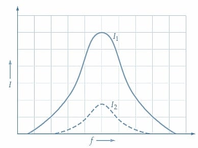
The frequency response curves of I₁ and I₂ for loosely coupled coils are shown in Figure 4(a). The shape of the I₁ response curve is largely unaffected by the coupled impedance, and the I₂ the curve is seen to be very much smaller than I₁ but with the same shape as the I₁ curve.

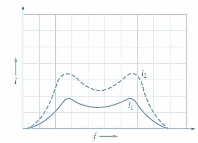
With tight coupling, as shown in Figure 4(b), the coupled resistance has a considerable effect at the resonance frequency. The total primary impedance is increased, and the primary current is significantly reduced. Also, the primary response curve is distorted by the occurrence of two humps: one above and one below the resonance frequency \((f_{r})\). These humps result from the fact that the secondary impedance is capacitive below the \(f_{r}\) and inductive above \(f_{r}\). When coupled into the primary, the coupled impedances are inductive below \(f_{r}\) and capacitive above \(f_{r}\). These result in minimum primary impedances and, therefore, maximum currents at two frequencies above and below resonance. Because of the tight coupling, the response curve of the secondary current is simply a slightly amplified version of the primary.

 

(a) Loose coupling.

 

(b) Tight coupling.

 

 

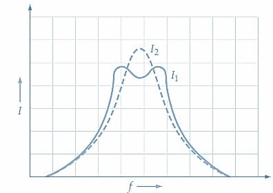
(c) Critical coupling.

Figure 4. The current-versus frequency response of tuned coupled coils depends on the degree of coupling. Loose coupling gives low secondary current, tight coupling produces distortion, and critical coupling affords maximum power transfer from primary to secondary. Image used courtesy of Amna Ahmad

 

With critical coupling, as shown in Figure 4(c), maximum power transfer occurs from the primary to the secondary; thus, the secondary current is greater than in the other two cases. The condition for maximum power transfer is that the source impedance and load impedance be equal. The two humps still occur in the primary response curve but are absent in the secondary.

For maximum power transfer and critical coupling

\[R_{1}=R^{{\,}'}_{2}=\frac{(\omega M)^{2}}{R_{2}}\]

Or

\[M^{2}=\frac{R_{1}R_{2}}{\omega^{2}}(10)\]

Where

\[M^{2}=k^{2}L_{1}L_{2}\]

Therefore

\[k^{2}L_{1}L_{2}=\frac{R_{1}R_{2}}{\omega^{2}}\]

Giving

\[k^{2}=\frac{R_{1}}{\omega L_{1}}\times\frac{R_{2}}{\omega L_{2}}=\frac{1}{Q_{1}}\times\frac{1}{Q_{2}}\]

For critical coupling

\[k=\frac{1}{\sqrt{Q_{1}Q_{2}}}(11)\]

 

Tuned Coupled Coils Takeaways

Tuned coupled coils are an interconnected arrangement of coils, designed to facilitate efficient energy transfer and signal transmission. Coupled impedance, a key characteristic, measures the impact of one coil's impedance on the other, influencing its overall performance. The coefficient of coupling quantifies the degree of magnetic coupling between the coils, providing valuable insights into their interdependent behavior.