National Electrical Code Basics: Computing Voltage Drop in Branch Circuits and Feeders Part 3

To catch up on the rest of Lorenzo Mari's series on computing voltage drop in branch circuits and feeders, follow these links:

• National Electrical Code Basics: Computing Voltage Drop in Branch Circuits and Feeders Part 1
• National Electrical Code Basics: Computing Voltage Drop in Branch Circuits and Feeders Part 2

Using Single-phase Voltage Drop Formulas and Tables in Three-phase Systems

Reducing the I²R losses and voltage drops in three-phase systems allows the use of smaller conductors, decreasing the weight of copper or aluminum required.

The formulas and tables employed to compute voltage drops in single-phase systems may be used in three-phase systems through multiplication by factors. The elaboration of these factors requires a review of a few three-phase basics.

Voltages in Balanced Three-phase Systems

Synchronous generators in utility power plants produce most of the power transmitted and distributed through lines operating as three-phase circuits.

These generators produce three sinusoidal voltages, with equal Root Medium Squared (RMS) magnitude and a phase shift of 120 electrical degrees among them. Since the voltages are sinusoidal, their representation uses phasors.

The system is balanced because they have equal RMS magnitudes. There are no unbalanced generators under normal operating conditions.

The three generated voltages can be connected either in a wye configuration or a delta configuration. The wye connection is typical in utility generators. Figure 1 shows both formats.

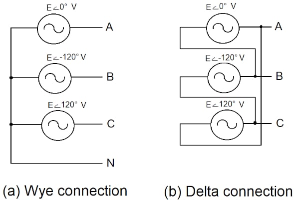
Figure 1. Balanced 3-phase voltage sources wye- and delta-connected. Image used courtesy of Lorenzo Mari

The Wye Connection

In the wye connection (figure 1a), three source terminals form a common node labeled the neutral (N).

The line-to-neutral system voltages, or phase voltages, are equal to the individual source voltages

V_AN = E 0ے°

\[V_{BN} = Eے-120° V\]

\[V_{CN}= Eے120° V\]

To determine the line-to-line voltages or line voltages, we apply the Kirchhoff Voltage Law (KVL)

\[V_{AB} = V_{AN} – V_{BN} = Eے0° - Eے-120° = √3Eے30° V\]

\[V_{BC} = V_{BN} – V_{CN} = Eے-120° - Eے120° = √3Eے270° V\]

\[V_{CA} = V_{CN} – V_{AN} = Eے120° - Eے0° = √3Eے150° V\]

Denoting the magnitude of the line voltage by V_L and the phase voltage by V_P, we have

V_L = √3 V_P

In the wye connection, the line voltage magnitude is √3 times the phase voltage. There is phase displacement between the line and phase voltages.

The Delta Connection

We get a delta connection by joining the three sources in series (figure 1b). The generator neutral is absent since the three sources do not have a common point. For instance, no line-to-neutral voltages exist, except for the line-to-ground capacitance (not covered in this analysis).

In the delta connection, the line voltages are equal to the individual phase voltages, as follows

\[V_{AB} = Eے0° V\]

\[V_{BC} = Eے-120° V\]

\[V_{CA} = Eے120° V\]

Then

V_L = V_P

Currents in Balanced Three-phase Loads

Figure 2 shows a generator’s three single-phase loads connected to phases A, B, and C.

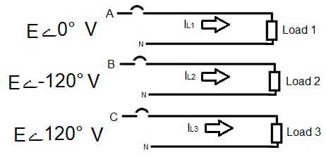
Figure 2. Single-phase loads connected to a generator. Image used courtesy of Lorenzo Mari

The three single-phase circuits have the currents IL1, IL2, and IL3, flowing from the source to the load and back to the source – assuming wye connected generator windings with the neutral connection accessible. Each neutral will carry current, and the single-phase voltage drop formulas will apply.

Similar to the sources, the three single-phase loads may be connected in wye or delta configurations (figure 3).

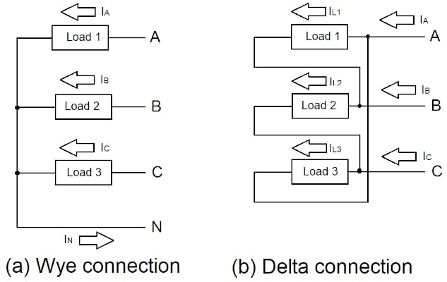
Figure 3. 3-phase loads wye- and delta-connected. Image used courtesy of Lorenzo Mari

The Wye-wye Connection

Figure 3a shows the three loads connected in wye. The term wye-wye means that the source and the load are wye-connected.

The voltages applied to the loads are equal to the source phase voltages.

The three impedances are equal in a balanced system. Assuming load impedances Z₁ = Z₂ = Z₃ = Z_P ےθ, Ohm’s law, gives the following phase currents

\[I_{A} = V_{AN}/Z_{P} ےθ = Eے0°/Z_{P} ےθ A\]

\[I_{B} = V_{BN}/Z_{P} ےθ = Eے-120°/Z_{P} ےθ A\]

\[I_{C} = V_{CN}/Z_{P} ےθ = V_{CN} = Eے120°/Z_{P} ےθ A\]

The currents in the three phases have the same magnitude and 120° phase displacement among them.

In each phase of a wye-wye connection, the line current equals the phase current in magnitude and phase. Denoting the magnitude of the line current by IL and the phase current by IP, we have

I_L = I_P = I

Applying Kirchhoff’s current law (KCL)

I_N = I_A + I_B + I_C = 0

The neutral current is zero in a wye-connected, balanced, three-phase system. Since the neutral carries no current in this symmetrical circuit, it may be ignored to establish a three-phase, three-wire system – although it is physically a four-wire system.

In our discussion about voltage drops, it is essential to have the circuit operating under balanced conditions. As a result, only one conductor feeds every load, producing only half the voltage drop that would occur under unbalanced conditions – with the phase and neutral carrying current.

The Wye-delta Connection

Figure 3b shows the three balanced loads connected in delta. The voltages applied to the loads are equal to the source line voltages. Systems with delta-connected loads are three-wire because there is no neutral connection.

The system is wye-delta or delta-delta depending on the source connection – wye- or delta-connected. Delta-connected sources are atypical, so we will adopt a wye-connected source.

Assuming load impedances Z₁ = Z₂ = Z₃ = Z_P ےθ, the phase currents are

\[I_{L1} = V_{AB}/ Z_{P} ےθ = √3Eے30°/Z_{P} ےθ A\]

\[I_{L2} = V_{BC}/ Z_{P} ےθ = √3Eے270°/Z_{P} ےθ A\]

\[I_{L3} = V_{CA}/ Z_{P} ےθ = √3Eے150°/Z_{P} ےθ A\]

With three like impedances, this is a balanced load with equal phase current magnitudes, displaced 120°.

Applying KCL to determine the line currents I_A, I_B, and I_C

I_A = I_L1 – I_L3

I_B = I_L2 – I_L1

I_C = I_L3 – I_L2

After some calculations we get

\[I_{A} = √3 I_{L1}ے-30° A\]

\[I_{B} = √3 I_{L2}ے-30° A\]

\[I_{C} = √3 I_{L3}ے-30° A\]

Then

I_L = √3 I_P

We conclude that the line current magnitude equals √3 times the magnitude of the phase current, and the line current lags 30° the phase current, assuming a positive sequence.

Multiplying Factors

Recall the typical formula to compute approximate voltage drop in single-phase circuits

VD = 2 x K x I_L x L / A

where

VD = voltage drop

K = conductor resistivity

I_L = line current (I_L= I_P in a single-phase circuit)

A = cross-sectional area of the conductor

L = distance from source to load

The constant 2 contemplates the return conductor from the load to the source

The criteria to find the multiplying factors are

a. The constant 2 should be removed since there is no return conductor (neutral) in delta-connected loads and balanced wye-connected loads – they are three-wire circuits.

b. In a delta-connected load I_L = √3 I_P. Substitute I_L by √3 I_P in the formula. With VD based on V_L, the factor is √3/2 = 0.866.

c. In a wye-connected load, V_L = √3 V_P.

c1. With VD based on V_L, divide VD by √3, and the factor is √3/2 = 0.866.

c2. With VD based on V_P, the factor is ½ = 0.5.

To summarize, in three-phase systems, multiply the single-phase result by 0.866 if using line voltages and by 0.5 if using phase voltages.

Example 1

Figure 4 shows a branch circuit supplying a delta-connected, low inductance load. Compute the three-phase voltage drop using the following single-phase formula for aluminum.

VD = 2 x 17.35 Ω CM/ft x I_L(A) x L(ft) /CM

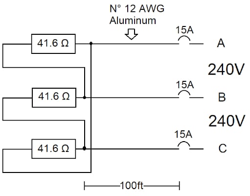
Figure 4. Balanced 3-phase delta-connected load. Image used courtesy of Lorenzo Mari

I_P = 240 V/41.6 Ω = 5.77 A

I_L = √3 I_P = 10 A

The NEC Table 8 shows 6 530 circular mils for conductor size N° 12 AWG.

VD = (2 x 17.35 Ω CM/ft x 10 A x 100 ft / 6 530) x 0.866 = 4.6 V

Example 2

Figure 5 shows a branch circuit supplying a wye-connected, low inductance load. Compute the size of copper wire for a voltage drop not higher than 1% based on V_P. Use the following single-phase formula for copper

CM = 2 x 10.895 Ω CM/ft x I(A) x L(ft) /VD(V)

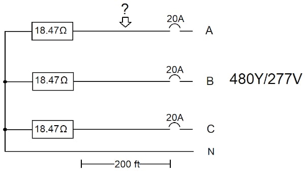
Figure 5. Balanced 3-phase wye-connected load. Image used courtesy of Lorenzo Mari

I = 277 V/18.47 Ω = 15 A

VD = 0.01 x 277 V = 2.77 V

CM = (2 x 10.895 Ω CM/ft x 15 A x 200 ft / 2.77 V) x 0.5 = 11 800

The NEC Table 8 shows 10 830 CM for N° 10 AWG and 16 510 for N° 8 AWG. Use N° 8 AWG.

Example 3

Repeat example 2 for a voltage drop not higher than 1% based on V_L.

I = 277 V/18.47 Ω = 15 A

VD = 0.01 x 480 V = 4.8 V

CM = (2 x 10.895 Ω CM/ft x 15 A x 200 ft / 4.8 V) x 0.866 = 11 800

Use N° 8 AWG.

The Proportional Method to Compute Voltage Drops

The following expressions are helpful to compute the voltage drop and phase shift due to the voltage drop along the conductors

V_R = V_S x Z_L/Z_S

where

V_R = phase voltage at the load

V_S = phase voltage at the source

Z_L = load impedance

Z_S = system impedance, including Z_L

All quantities expressed phasorially

The magnitude of the voltage drop is

ƖVDƖ = ƖV_SƖ – ƖV_RƖ

Example 4

Figure 6 shows a source supplying power to an apparatus with a power factor different from 100%.

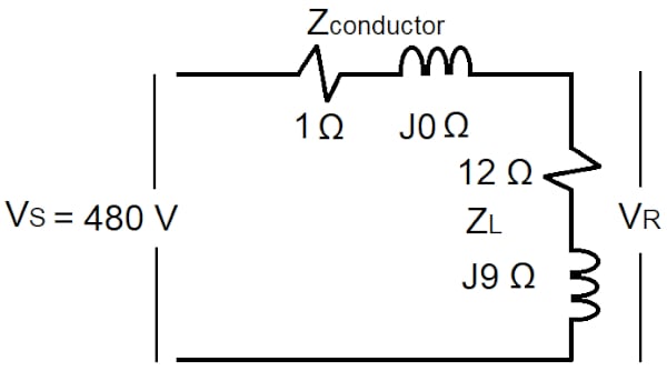
Figure 6. Source feeding an apparatus. Image used courtesy of Lorenzo Mari

a. Compute Z_L in polar form.

The format for the polar form is

ƖZ_LƖ ےθ

ƖZ_LƖ = √(12² + 9²) = 15 Ω

θ = tan¯¹ 9/12 = tan¯¹ 0.75 = 36.9°

\[Z_{L} = 15 ے36.9° Ω\]

b. Compute Z_S in rectangular and polar forms.

The format for the rectangular form is

Z_S = R + jX

Z_S = 1 + j0 + 12 + j9 = 13 + j9 Ω

ƖZ_SƖ = √(13² + 9²) = 15.81 Ω

θ = tan¯¹ 9/13 = tan¯¹ 0.69 = 34.7°

\[Z_{S} = 15.81ے 34.7° Ω\]

c. Compute the voltage at the load. Select VS as the reference.

\[V_{R} = 480 ے0° \times 15 ے36.9°/15.81ے 34.7° = 455.4 ے2.2° V\]

d. Compute the voltage drop magnitude in volt and percentage.

ƖVDƖ = 480 V – 455.4 V = 24.6 V

24.6 V/480 V x 100 = 5.13%

e. What’s the phase shift introduced by the conductor?

2.2°

f. Compute the apparatus load factor.

P.F. = cos θ = cos 36.9° = 0.8 = 80% lagging

A Typical Approximate Formula Used in Three-phase Circuits

Only one phase is required to determine the voltage drop in a three-phase system operating under balanced conditions. The phasor diagram of figure 7 shows the single-phase voltages at the source, the load, and the conductor (closing the loop).

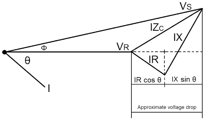
Figure 7. Single-phase phasor diagram for voltage drop calculations. Image used courtesy of Lorenzo Mari

The projection of the conductor voltage on the real axis approximates the voltage drop magnitude. The result is

ƖVDƖ = I (R cos θ + X sin θ)

where

ƖVDƖ = magnitude of line-to-neutral voltage drop

I = magnitude of line current

R = conductor resistance 

X = conductor reactance

θ = load angle

cos θ = load power factor

sin θ = load reactive factor

The formula error lessens as the angle Φ approximates zero – the formula is exact for Φ = 0. In practice, the angle Φ is small.

Modifying this equation to calculate the voltage drop in percentage directly, we get

VD% = kVA (R cos θ + X sin θ) /10 kV²

where

VD% = voltage drop in percentage

kVA = three-phase apparent power

kV = line voltage

Notice that kVA and kV are three-phase values.

Example 5

a. Using the approximate formula and the results of example 4, compute the voltage drop magnitude in the figure 6 circuit.

\[I = 480 Vے0°/15.81ے34.7° = 30.36ے-34.7° A\]

The magnitude of line current = 30.36 A

Z_L angle = θ = 36.9°

R = conductor resistance = 1 Ω

X = conductor reactance = 0 Ω

cos θ = load power factor = 0.8

sin θ = load reactive factor = 0.6

ƖVDƖ = 30.36 x (1 x 0.8 + 0 x 0.6) = 24.29 V

b. Calculate the percent voltage drop.

24.29 V/480 V x 100 = 5.06%

c. Calculate the voltage drop in percentage directly.

Apparent power = 30.36 A x 0.48 kV = 14.57 kVA

VD% = 14.57 (1 cos 36.9° + 0 sin 36.9°) /10 x 0.48² = 5.06%

Example 6

A three-phase underground cable supplies power to a balanced inductive load (lagging power factor). System data are as follows

Cable impedance ZC = 0.0771 + j0.0724 Ω/phase

Load impedance ZL = 13.75 + j10.31 = 17.19 ے36.86° Ω/phase

Source voltage 4.16Y/2.4 kV

a. Determine the voltage drop using the proportional method.

V_R = V_S x Z_L/Z_S

\[Z_{S} = Z_{C} + Z_{L} = 0.0771 + 13.75 + j(0.0724 + 10.31) = 13.83 + j10.38 = 17.29
ے36.9° Ω/phase\]

Selecting the phase voltage as the reference

\[V_{S} = 2 400 ے0° V\]

\[V_{R} = 2 400 ے0° \times 17.19 ے36.86°/ 17.29 ے36.9° = 2 385.4 ے-0.04°\]

\[ƖVDƖ = 2 400 V – 2 385.4 V = 14.6 V\]

\[14.6 V/ 2 400 V x 100 = 0.61%\]

b. Determine the voltage drop using the approximate formula.

ƖVDƖ = I (R cos θ + X sin θ)

Z_L angle = θ = 36.86°

R = conductor resistance = 0.0771 Ω

X = conductor reactance = 0.0724 Ω

cos θ = load power factor = 0.8

sin θ = load reactive factor = 0.6

\[I = V_{S}/Z_{S} = 2 400 ے0° /17.29 ے36.9° = 138.72 ے-36.9° A\]

The magnitude of line current = 138.72 A

ƖVDƖ = 138.72 (0.0771 x 0.8 + 0.0724 x 0.6) = 8.56 + 6.03 = 14.6 V

c. Calculate the voltage drop in percentage directly.

VD% = kVA (R cos θ + X sin θ) /10 kV²

Line voltage = V_L = 4.16 kV

3-phase kVA = √3 x V_L x I = √3 x 4.16 kV x 138.72 A = 1 000 kVA

VD% = 1 000 (0.0771 x 0.8 + 0.0724 x 0.6) / 10 x 4.16² = 0.61%

Summary

Large residential complexes and commercial and industrial facilities employ three-phase systems to supply significant power.

The application of factors allows single-phase methods to calculate voltage drops in three-phase systems.

This article reviews some typical methods to determine voltage drops in three-phase systems.

Featured image used courtesy of Pexels