Modeling Medium and Long Transmission Lines for Power System Analysis

The first article in this series provided the basic framework for transmission line modeling by explaining how accurate line models impact power system analysis. It described the importance of incorporating series impedance, shunt admittance, and distributed parameters in the transmission line models, and applied that to short transmission lines. Now, this article will examine the models for medium and long transmission lines.

Medium Transmission Line Model (80–250 km)

Medium-length transmission lines—typically spanning distances from 80 to 250 kilometers and operating at voltages between 132 kV and 230 kV—represent a transitional domain in power system modeling. At these lengths, the distributed nature of line capacitance begins to noticeably influence voltage profiles and reactive power behavior, especially under light-load or open-circuit conditions.

However, fully distributed-parameter models are not yet necessary; instead, lumped-parameter approximations such as the nominal π-model and nominal T-model provide an effective balance between computational efficiency and physical accuracy.

Inclusion of Shunt Capacitance

Unlike short lines where shunt admittance is negligible, medium lines exhibit significant line charging current and voltage rise at the receiving end, requiring inclusion of the line’s capacitive effects. These effects are approximated using lumped shunt capacitors connected at one or both ends of the line. The shunt admittance Y = jωC is derived from the per-unit-length capacitance of the line, scaled by its total length.

For symmetrical lines, the total shunt admittance Y is typically split equally and placed at both ends (π-model), or grouped at the line’s midpoint (T-model). This simplifies the otherwise distributed behavior of capacitance without introducing large errors in voltage or current predictions.

Nominal π Model Formulation

The nominal π-model is the most commonly used representation for medium lines. It models the transmission line as a lumped series impedance Z = R + jωL and splits the shunt admittance Y = jωC equally between the sending and receiving ends.

The ABCD parameters for the nominal π-model are:

$$A = D = 1 + \frac{YZ}{2}$$

$$B = Z$$

$$C = Y(1 + \frac{YZ}{4})$$

These parameters are used in the standard transmission line equations:

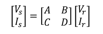
where:

• V_s and V_r are the sending and receiving end voltages
• I_s and I_r are the sending and receiving end currents.

This formulation enables the evaluation of voltage regulation, sending-end power requirements, and line efficiency under various loading conditions.

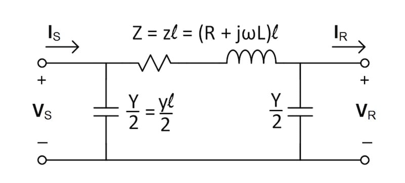
Figure 1. Medium transmission line model. Image used courtesy of Oregon State University

Voltage Regulation and Charging Current

In open-circuit or light-load conditions, the charging current drawn by the shunt capacitance can lead to a phenomenon known as Ferranti Effect, where the receiving end voltage V_r exceeds the sending end voltage V_s. This occurs due to reactive power injection from the line’s capacitive elements, and is quantified using voltage regulation:

$$\text{Voltage Regulation} = (\frac{V_s - V_r}{V_r}) \times 100 \%$$

For lightly loaded lines, this can be positive or even negative, depending on the degree of capacitive charging. The charging current I_c itself can be approximated as:

$$I_c = j \omega CV_r$$

Where C is the total capacitance seen from the receiving end. Accurate modeling of this behavior is essential in systems with long transmission corridors or low-load rural feeders.

Nominal T Model (Less Common)

The T-model provides an alternative where the shunt admittance is lumped at the midpoint rather than at the ends. Its ABCD parameters are slightly different but suitable for certain analytical applications. However, due to its less accurate approximation of terminal behavior compared to the π-model, its usage is limited in modern power flow and stability programs.

Long Transmission Line Model (> 250 km)

For lines longer than roughly 250 km and operating at 345 kV and above, the distributed physical nature of the line must be accurately modeled. Unlike short and medium lines where the line constants are lumped at discrete points, long lines exhibit continuous electrical behavior along their length. Each differential segment contributes to voltage drop and current change, requiring the use of the telegrapher’s equations for an accurate representation. These are a pair of coupled, linear, first-order differential equations:

$$\frac{dV(x)}{dx} = - (R + j\omega L)\cdot I(x)$$

$$\frac{dI(x)}{dx} = - (G + j\omega C)\cdot V(x)$$

Solving these yields a set of second-order wave equations for voltage and current. The general solution describes wave propagation in both directions along the line:

$$V(x) = V_+e^{- \gamma x} + V_-e^{\gamma x}$$

$$I(x) = \frac{V_+}{Z_0}e^{- \gamma x} - \frac{V_-}{Z_0}e^{\gamma x}$$

These equations form the foundation of the long-line model, allowing engineers to account for attenuation, phase shift, and reflection effects in high-voltage transmission analysis.

Propagation Constant and Characteristic Impedance

The term γ is the propagation constant and encapsulates both the attenuation (real part α) and phase shift (imaginary part ꞵ) per unit length. It is defined as:

$$\gamma = \alpha + j \beta = \sqrt{(R + j\omega L)(G + j\omega C)}$$

The characteristic impedance Z₀, which determines the relationship between traveling voltage and current waves, is given by:

$$Z_0 = \sqrt{\frac{(R + j\omega L)}{(G + j\omega C)}}$$

These parameters are especially critical when modeling systems with low-loss overhead lines, where reflections due to mismatched impedances can affect both voltage regulation and protection coordination.

For a lossless line, i.e., when R = 0 and G = 0, the propagation constant simplifies to a purely imaginary quantity and the characteristic impedance becomes purely real:

$$Z_0 \approx \sqrt{\frac{L}{C}}$$

$$\gamma = j \omega \sqrt{LC}$$

This idealized condition is often used in initial analyses or when conductor resistance and dielectric losses are negligible.

Hyperbolic-Function Form and ABCD Parameters

For practical power system studies, it is useful to represent the long line as a two-port network characterized by ABCD parameters. By solving the voltage and current expressions at both sending and receiving ends and applying boundary conditions, we obtain the ABCD parameters in terms of hyperbolic functions:

$$A = D = \cosh(\gamma l)$$

$$B = Z_0 \sinh(\gamma l)$$

$$C = \frac{\sinh(\gamma l)}{Z_0}$$

This representation maintains the distributed nature of the line while enabling simplified analysis in network-level studies. These parameters are crucial in calculating sending-end quantities, line losses, voltage regulation, and transient stability margins in simulation software such as PSCAD or PowerWorld.

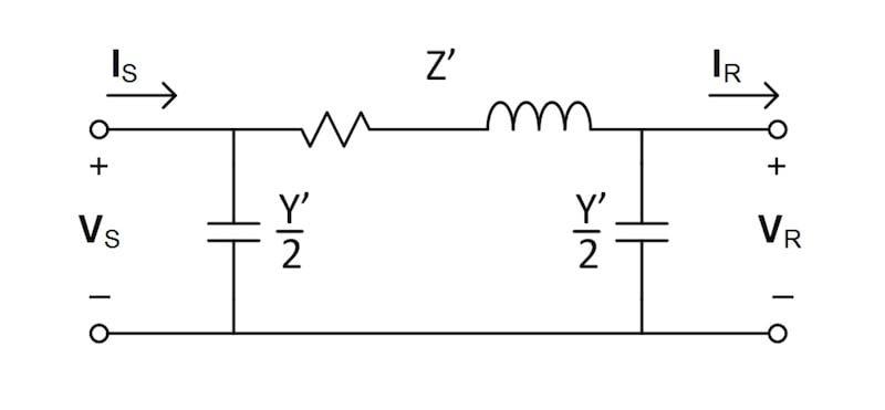
Figure 2. Long transmission line equivalent π model. Image used courtesy of Oregon State University

Practical Implications

The practical impacts of long-line behavior become significant under both light and heavy load conditions. Under light loads, the shunt capacitance causes the Ferranti effect, whereby the receiving-end voltage exceeds the sending-end voltage due to excess charging current. In contrast, under high load, the phase angle difference across the line increases, reducing synchronizing power and risking angular instability.

Additionally, the line's distributed nature can affect fault detection and relay operation, as traveling wavefronts do not instantaneously propagate. This requires the use of advanced protection schemes like traveling wave relays or distance relays that compensate for line propagation delay.

Long-line models also aid in evaluating resonance phenomena such as subsynchronous resonance (SSR), where interaction between turbine-generator shafts and line capacitive reactance can lead to mechanical stress and failure. Inclusion of Z₀ and γ in the transmission system's equivalent circuits is therefore essential for accurate dynamic and steady-state analysis.

Key Takeaways

As we have seen in this article series, each line model—short, medium, and long—serves a distinct purpose depending on physical length and voltage level. As distances increase, there is increased emphasis on distributed parameters. As utilities transition to smarter and more adaptive grid operations, rigorous transmission line modeling becomes foundational to achieving resilience, operational flexibility, and secure energy delivery across interconnected networks.

Featured image used courtesy of Adobe Stock (licensed)