Facebook
 Google
 GitHub
 Linkedin
Grounding and Bonding for High-Frequency Stimulus
Learn about the behavior of grounding and bonding conductors with high-frequency signals
With the proliferation of complex electronic equipment, high-frequency grounding and bonding have become an unavoidable concern of many electrical and electronic designers, installers, and users.

Image courtesy of Pixabay.
The speed of electronic circuits increase at a considerable rate. These increased speeds augment the complexity of the grounding networks. A grounding design that was adequate a few years ago might be unacceptable when used with the faster components available today. The problem can be significant when older, slower parts cease to be obtainable. A more rapid part, designed to supersede an older one, may fail to operate correctly with the existing grounding and bonding system.
It is effortless to overlook correct grounding and bonding in system design, though every electrical engineer knows their basics. Neglecting proper grounding and bonding may cause equipment malfunction that may range from a simple annoyance to a major disaster, often requiring expensive repairs.
To design proper high-frequency grounding systems, the engineers must understand specific specialized topics such as transmission line theory and antenna theory. The impulses that affect electronic equipment are usually short duration and fast transition, requiring the analysis of the grounding and bonding conductors’ behavior through transmission line theory.
It is almost impossible to design a universal method that will work for every conceivable situation. But some basic concepts and guidelines provide a reasonable degree of confidence for typical installations. In general, it is an excellent practice to follow the equipment manufacturer’s guidelines as to how to install the grounding system, but with due caution because the specifications may not be precise, allowing various interpretations by installers and users.
Each system requires a particular high-frequency grounding and bonding design. Its ideal objective is to provide a zero-volt reference system that limits the amount of electrical noise passing through a specific electronic equipment’s internal logic circuitry, avoiding the processed data’s corruption
Some disturbances are radio frequency interference (RFI), electromagnetic interference (EMI) – the higher the speed of an electronic component, the greater the likelihood of EMI – and electrical impulses caused by electric motors, variable speed drives, welders, and other industrial devices. Electromagnetic compatibility (EMC) is the capability of two or more electrical devices to operate together without mutual interference. An apparatus susceptible to undesired noise will usually not perform satisfactorily. Modern electronic equipment minimizes stray emissions and tolerates high levels of inflicted noise.
As usual, compliance with the National Electrical Code’s (NEC) safety rules is a must. By no means should the equipment manufacturer´s installation requirements be followed if they violate the NEC. An NEC violation might injure people and damage property.
Useful Terms
Waveform: The path traced by a quantity, like voltage and current, plotted as a function of a variable such as position and time.
Periodic waveform: A waveform that repeats itself after the same time interval.
Period (T). The time interval between repetitions of a periodic waveform. Expressed in seconds.
Cycle: That portion of a waveform contained in one period of time.
Figure 1 shows one period and one cycle for a sinusoidal wave.

Figure 1. One period and one cycle of a sinusoidal wave.
Frequency (f): The number of cycles in a unit of time, usually expressed in Hertz (Hz). 1 Hz = 1 cycle per second. f=1/T or T=1/f.
Figure 2 shows a sinusoidal wave with a frequency of one cycle per second or one Hz.

Figure 2. A frequency of 1 Hz.
Radian (rad): A unit to measure an angle, frequently used in work with electrical circuits, equivalent to 57.3°. 360° = 2∙π rad. Figure 3 shows a sine wave using the radian as the unit of measurement for the abscissa.

Figure 3. Sine wave using radians.
Wavelength (ʎ): The periodic waveform size measured as the distance between two similar points over the wave – the distance where the phase changes by 2∙π rad. Figure 4 shows a sine wave using the distance as the unit of measurement for the abscissa.

Figure 4. Sine wave using distance.
In a lossless transmission line ʎ=c/f, where c = speed of electromagnetic waves in the ambient medium, and f = frequency. In free space, c = speed of light = 300,000km/s. In many applications, the ambient medium is not free space or air, as in cables and rotating machines, lessening the propagation speed.
Transmission line: An arrangement of conductors to facilitate the transfer of electromagnetic energy between two points.
Lumped circuit: A circuit with inductance concentrated in a coil, capacitance in a capacitor, and resistance in a resistor. Such a circuit has lumped constants.
Distributed circuit: A circuit with inductance, capacitance, and resistance distributed along the wire. Such a circuit has distributed constants.
Traveling Waves on Transmission Lines
It is feasible transferring electromagnetic energy as traveling waves between two places. One of the essential requirements in transmission lines is moving energy between two points without radiation loss, which involves transporting electromagnetic energy in a propagating wave.
Transmission lines have resistance, inductance, and capacitance distributed along their length. An attractive property is that each meter of distance is much like every other meter. This property gives them the ability to support traveling waves of current and voltage.
Figure 5 shows a switch S closing at t = 0 connecting a V volt dc battery – with zero resistance – to a transmission line feeding a given remote load.

Figure 5. Battery supplying a load through a transmission line.
To describe what happens when the switch S closes, it helps treat the events as electromagnetic boundary-value problems, emphasizing a field point of view.
The electromagnetic pulse created by closing S does not appear instantaneously along the line but travels with a finite speed and arrives at the load after an interval determined by the speed of propagation of the medium’s electromagnetic waves surrounding the line.
After energizing the circuit, the traveling wave of voltage passing along the line establishes an electric field between the conductors as it does so. The voltage wave is accompanied by a current wave, which creates a magnetic field in the surrounding space.
The speed of propagation is independent of the line geometry.
Let’s now apply a 100 MHz voltage source to a transmission line. Assuming c = 300,000km/s, the wavelength is ʎ = c/f = 300/100 = 3m, and the period T= 1/f = 1/100X106 = 0.01 µs. It means that a complete cycle takes 0.01µs, and will be present along every 3 m of the line — a distance of one wavelength.
Figures 6 and 7 show the voltage’s period and wavelength.
Figures 8 to 11 show instantaneous positions of the voltage wavefront traveling along the line at several time intervals.

Figure 6. Period.

Figure 7. Wavelength.

Figure 8. Wavefront position after t = 0.0025µs (ʎ4).

Figure 9. Wavefront position after t = 0.005µs (ʎ2).

Figure 10. Wavefront position after t = 0.0075µs (34ʎ).

Figure 11. Wavefront position after t = 0.01µs (ʎ).
About Grounding and Bonding Behavior for High-Frequency Stimulus
A correct ground connection is a crucial factor for the error-free operation of electronic equipment. High-frequency grounding and bonding are significant design issues in most electronic systems that must be designed and implemented with judgment.
With the introduction of electronic equipment types, many grounding and bonding problems became evident. Several difficulties resulted because the circuit and equipment grounds often provide a mechanism for noise coupling.
The grounding arrangements contemplate the circuit’s dimensions and frequencies in use.
Analyzing the grounding and bonding conductors as transmission lines is the best way to understand their high-frequency behavior. The voltages and currents along a uniform ground path are a function of time and distance, and its impedance is equivalent to that offered by a short-circuited transmission line. The voltage and current do not appear instantaneously along the line but propagates with a finite speed.