Facebook
 Google
 GitHub
 Linkedin
Differential Mode Vs. Common Mode Conducted Emissions
The article presented the basic knowledge about conducted emissions providing an essential and intuitive overview, starting from how they are generated and later discussing measurement techniques and filtering.
Every time you connect a device to a power supply, there are two types of currents conducted through the power cable: differential mode currents and common mode currents. The sum of such currents is measured during a conducted emissions test and its spectrum is compared with limits.
Differential mode currents are those normally generated by the device in order to power the device. They can be also referred to as the supply currents, which generally speaking can be composed of low frequencies (i.e. 50/60Hz) and high frequencies (i.e. 100KHz + harmonics of a switching circuit).
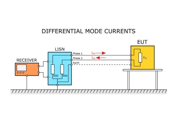
Figure 1. Differential mode currents in the conducted emissions test
Common mode currents are usually neglected due only to the parasitic parameters of the whole system, not only to the ones of the device itself.
Consider this question: Do you remember the 50/60Hz signal that you see on the scope when touching the probe with your finger? It is due to a phenomenon similar to common mode currents: a source generates a field (50/60Hz from the building cables) that through parasitic parameters couples with your body, that in turn conducts the coupled voltage to the probe and the scope.
The scope is coupled to the public line again through its internal parasitic parameters and power cable. In the end, it is generated a large loop that is able to conduct a small current determined by the architecture of devices in the system, the associated parasitic parameters, and signal sources in the system (voltage of the building cables and voltages of the circuit inside the scope).
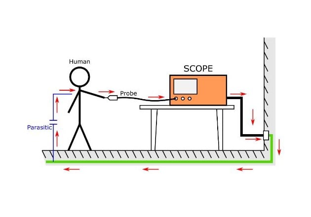
Figure 2. The measure of the signal produced when touching the probe with a finger.
A similar situation happens during the test of conducted emissions. Both lines of the main supply can conduct a current in the same direction that couples with the chassis of the EUT at RF. The chassis is connected to the earth cable that in this scheme works as a return path for such common mode currents, creating a loop.
Common mode currents can be present also if the UT is not connected to the earth or it doesn’t have a conductive chassis, because the internal circuit of the EUT can couple directly to the ground plane below the EUT itself.
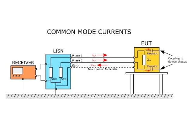
Figure 3. Common mode currents in the conducted emissions test.
The receiver measures the voltage across the 50Ω impedance presented at RF by the LISN on each phase. Summing the differential and common mode currents, the resulting measured signals at the receiver are:
-
VPHASE1 = 50Ω ∙ (ICM + IDM)
-
VPHASE2 = 50Ω ∙ (ICM - IDM)
Usually, such voltages are measured at the receiver as dBuV in order to compare them to the limits provided by the EMC regulations, as illustrated before.
Noise Reduction Techniques
Each device requires some kind of filtering at the mains port in order to reduce the differential and common mode currents at the LISN, thus keeping total measured noise below the limits.
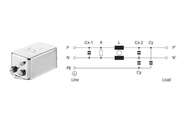
Figure 4. General-purpose AC/DC EMI filter. Image courtesy of SCHAFFNER FN2020 datasheet
A very common scheme for filtering is the one presented in Figure 4. Capacitors across the phases (Cx-1 and Cx-2) at RF present a low impedance that works as filters for differential mode currents. Instead, the capacitors Cy between each phase and earth connection PE, make the role to short the common mode currents to the earth connection avoiding them to reach the LISN phases, so working as common mode filters.
L is a common mode choke, a kind of transformer where each winding is in series with each line. For the currents that have the same direction (common mode), the impedance presented is very high and L works as a filter. On the contrary, for the currents that have opposite directions (differential mode), the impedance presented is very low and the effect of L is negligible.
Around this common scheme, there are many variants and designers work to adapt the filtering stage to the specific case of the device.