 Facebook
 Google
 GitHub
 Linkedin
Static vs. Dynamic ZIP Loads in IEEE Power Testing
Learn how dynamic and static ZIP loads affect power flow and stability in IEEE test systems using impedance, current, and power models.
The accuracy of power analysis greatly relies on realistic modeling. To achieve this, researchers and power engineers employ a composite model, referred to as the ZIP model, that merges three elements: impedance (Z), constant current (I), and constant power (P). The ZIP model efficiently simulates real-world loads and behavior, predicting how they respond to fluctuations in voltage.
In standard IEEE test systems, such as the IEEE 14-bus and IEEE 39-bus (New England) systems, modeling ZIP loads is crucial for assessing the performance and stability of the system. The two types of ZIP loads are static, characterized by the immediate response, and dynamic loads, which take time to react.
Understanding the difference between the two types of loads is crucial for conducting accurate load flow analysis, developing power control strategies, and ensuring transient stability in modern power systems.
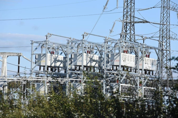
Figure 1. High-voltage substations which use ZIP load models at bus nodes for power flow and dynamic stability analyses in IEEE test systems. Image used courtesy of Unsplash.
Understanding ZIP Loads
To understand the load components in power systems, it is essential to consider that their behavior varies across different loads within the system. For this reason, a weighted combination of Z, I, and P components practically shows the response of the load's behavior as the voltage changes within the power system.
Constant impedance load (Z) in the ZIP model analyzes the passive electrical impedance by following Ohm's law and obeying the quadratic relation between the power consumed and the system voltage. To determine the actual power resulting from a constant impedance load (Pz), the instantaneous voltage at the load terminal (V) and the load resistance (R) is taken into account.
$$P_Z = \frac{V^2}{R}$$
When per unit form is considered relative to the nominal conditions, the constant impedance in the ZIP model is scaled as shown below, in which (V0) is the nominal voltage, V is the actual voltage, and P0 is the nominal power.
$$\frac{P_Z}{P_0} = \big( \frac{V}{V_0} \big)^2$$
For instance, if there is a 10% voltage drop, in which V/V0 = 0.9, the power drawn as a result of constant impedance can be scaled to decrease the drawn power by 81% of the original power, as shown here:
$$P_Z = P_0 \times (0.9)^2 = 0.81P_0$$
When it comes to understanding the constant current load (I), also referred to as a linear voltage-dependent, in ZIP load modeling, there is a linear increase in power consumption as the voltage increases, meaning the load remains proportional to the voltage in the system. To therefore determine, the power drawn (PI) as a result of constant current per unit voltage (V/V0) and the nominal power (P0) is considered.
$$P_I = P_0 \times \big( \frac{V}{V_0} \big)$$
For instance, consider a 1000W load at a nominal voltage V0, that has a 90% nominal voltage drop (V/V0 = 0.9), then:
$$P_I = 1000 \times 0.9 = 900 \text{ W}$$
If there is a 10% increase in the nominal voltage, the resultant power drawn increases proportionally, as shown in Figure 2.
$$P_I = 1000 \times 1.1 = 1100 \text{ W}$$
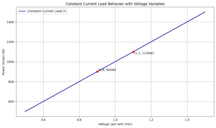
Figure 2. Graph showing the direct proportionality of constant current load and voltage variation. Image used courtesy of Bob Odhiambo.
Finally, the constant power load (P) in ZIP models maintains a fixed amount of real power consumption regardless of fluctuations in the supply voltage (Pp = P0). To achieve this, the drawn current is adjusted, with sudden voltage drops characterized by corresponding adjustments in current, ensuring the drawn power remains constant within the system.
To mathematically represent the behavior of loads in real-world power systems with voltage fluctuations, the ZIP formula is used where a1, a2, and a3 are the coefficients representing fractions of the three ZIP components. Instantaneous voltage V and the actual power consumed by the load in the power system P are considered for any given bus.
For normalized conditions, the sum of all coefficients equals one, ensuring that the total load equals P0 and the nominal voltage V equals V0. Therefore, the total real power resulting from ZIP load component behavior is expressed as:
$$P = P_0 \times \big[a_1 \big( \frac{V}{V_0} \big)^2 + a_2 \big( \frac{V}{V_0} \big) + a_3 \big]$$
Static vs Dynamic ZIP Loads in IEEE Testing
In determining steady-state operating conditions, a static ZIP model is employed, where, despite the load being directly influenced by voltage, there is no time-dependent response. For this reason, static ZIP loads feature instantaneous and proportional responses to changes in voltage without any time delay or sensitivity to changes in frequency.
To determine the real power consumption with voltage changes from its nominal value, the standard ZIP load formula is used. For instance, in the IEEE 14-bus system, each bus is assigned a ZIP coefficient (a1, a2, and a3) that represents the fractions of Z, I, and P of the total load.
When using the Newton-Raphson technique to solve for power flow, load power is adjusted based on the current bus voltage using the ZIP equation. This enables the evaluation of more precise power flow and voltage profiles, accurately representing the load's behavior in response to voltage changes within the power grid.
The static ZIP load model is, therefore, useful in routine planning studies, such as contingency analysis, load flow analysis, and optimal power flow calculations. As they ignore time-dependent behaviors, static models are efficient and faster, making them well-suited for large-scale planning studies.
On the other hand, Dynamic ZIP loads incorporate the time-domain behavior into the ZIP model, making them suitable for detailed simulation of system disturbances and transient stability studies in IEEE test systems. Evaluating not only the instantaneous response of the load to voltage changes but the dynamic model also captures the load's dynamic reaction to events like faults and fluctuations in frequencies, and even sudden trips in power generators over time.
The dynamic ZIP load model can also incorporate advanced features, such as delayed recovery from voltage sags, thermal protection, frequency-dependent load shedding, and motor stalling. In an IEEE 39-bus system, some buses may feature motor load models with dynamic ZIP characteristics that account for post-fault recovery delays and their response to variations in system frequency and voltage.
Following disturbances such as faults in three-phase motors, dynamic ZIP load models enable the simulation of aspects like potential load disconnection, delayed power restoration, and system damping effects, making them suitable for assessing not only voltage and frequency response but also the margins of power system stability.
| Feature | Static ZIP Load | Dynamic ZIP Load |
| Simulation Type | Steady-State Power Flow | Transient Stability |
| Time Dependence | No | Yes |
| Response to Faults | Instantaneous only | Captures recovery, delay, damping |
| Frequency Sensitivity | No | Yes (optional model) |
| Typical IEEE Test System Usage | IEEE 14-bus, 57-bus | IEEE 39-bus, 118-bus |
| Simulation Tools | PSS E, PowerWorld | PSS E (dynamic), PSCAD, DIgSILENT |
Table 1. Summary of the comparison factors of the static and dynamic ZIP load models.
Real World Relevance in Modern IEEE Test Applications
IEEE test systems utilize power flow studies using ZIP models to aggregate diverse loads, including residential, industrial, and commercial HVAC systems. Areas such as inverter-based distributed resources and smart grid controls, including demand response or DER dispatch, are better validated using realistic ZIP models.
Comparing the two ZIP models mentioned above, Power engineers and researchers can, therefore, employ static ZIP for routine planning. At the same time, dynamic ZIP is used for emergency operations and protection of power systems. Both models are helpful in grid modernization, ensuring stability and efficiency in power transmission.


This article delivers a clear and insightful explanation of ZIP load modeling in IEEE systems. I especially appreciated the way it breaks down the impact of each component, Z, I, and P, on power flow under voltage variations. The comparison between static and dynamic ZIP loads was not only informative but also practical, especially in the context of transient stability and fault response. The examples and equations made it easy to follow, even for complex scenarios like delayed recovery and motor stalling. Great job, Bob, this is a valuable read for anyone in power systems engineering.