Facebook
 Google
 GitHub
 Linkedin
Grid-Connected Inverter Modeling and Control of Distributed PV Systems
This article examines the modeling and control techniques of grid-connected inverters and distributed energy power conversion challenges.
Due to renewable energy’s intermittency, it must be stabilized. This is where power electronics devices like converters are crucial in ensuring the proper integration of renewable energy into the grid. Power electronics are vital in integrating distributed energy resources (DER) into the grid to manage and distribute power efficiently.

Image used courtesy of Adobe Stock
DER systems experience harmonic distortion and voltage fluctuation that can affect power in the grid and connected devices. Stabilization and optimization can be complex and challenging, requiring power electronics converters to improve power quality and minimize these issues.
The AC power in the grid can be a variable DC output of a renewable source converted by the power electronic converters. These converters can also adjust frequency and voltage in the grid network. These power electronics devices can also efficiently manage energy from batteries and supercapacitors.
Grid-Connected Inverter Modeling
There are several methods of modeling grid-connected inverters accurately for controlling renewable energy systems.
Space State Model
When modeling grid-connected inverters for PV systems, the dynamic behavior of the systems is considered. To best understand the interaction of power in the system, the space state model (SSM) is used to represent these states. This model is mathematically represented in an expression that states the first order of the differential equation. To understand how this method can be used in modeling, we will consider two important SSM variables for a single-phase grid-connected inverter, the states of the output current of the inverter and the DC-link voltage, to express a simplified space state model.
The state equations for the DC-link voltage and the inverter output current can be represented using the following formula:
\[v_{dc}=\frac{1}{C}(P_{in}-P_{out}-R\times I_{dc}^{\,\,\,\,\,2})\]
\[i_{dc}=\frac{1}{L}(V_{dc}-V_{grid})\]
where C represents the capacitance of the DC-link voltage.
R represents the value of resistance in the inverter’s DC circuit.
L represents the value of inductance of the output filter of the inverter.
Vgrid represents the constant voltage in the grid.
Pin is the power output from the PV array fed to the inverter.
Pout represents the power being provided to the grid.
To calculate the power output Pout use the formula below:
\[P_{out}=V_{dc}\times I_{dc}\]
SSM can best be represented in simulation software in which precise calculations can be carried out to update important parameters at each step of the simulation cycle. Consider the following parameters in the following example calculation states of DC-link voltage and inverter output current.
Assuming the initial DC-link voltage in a grid-connected inverter system is 400 V, R= 0.01 Ω, C = 0.1F, the first-time step i=1, a simulation time step Δt of 0.1 seconds, and constant grid voltage of 230 V use the formula below to get the voltage fed to the grid and the inverter current where the power from the PV arrays and the output provided to the grid are dynamic variables.
\[v_{dc}[i]=v_{dc}[i-1]+\frac{(P_{in}-P_{out}-R\times I_{dc}[i-1]^{2})}{C}\times\Delta t\]
Substitute the available parameters and variables to the formula to calculate the DC-link voltage:
\[v_{dc}[1]=400+\frac{(P_{in}-P_{out}-0.01\times I_{dc}[0]^{2})}{0.1}\times0.1\]
The inverter output current can be calculated using:
\[i_{dc}[i]=\frac{(V_{dc}[i]-V_{grid})}{L}\]
\[i_{dc}[1]=\frac{(V_{dc}[1]-230)}{0.1}\]
Pin and Pout variables are not included in the above calculations as they are dynamic and are represented in the simulation results below. According to the graphs in Figure 1 below, the simulation of the constant power of the PV arrays has been done in a range of 800 to 1200 W, and the output power fed to the grid varies between 700 and 1000 W in which the DC-link voltage and inverter current can be monitored over time.

Figure 1. SSM simulation of the state of DC-link voltage and the inverter output current. Image used courtesy of Bob Odhiambo
Other variables like voltage, current, and control signals are used to control the operation of the inverters and are included in the SSM. Apart from implementing the space-state model, there is a need to implement a control strategy to ensure the inverter’s operation is optimal and efficient. These control techniques include proportional-integrated derivative (PID) control, model predictive control (MPC), and sliding model control.
Transfer Function Model
A transfer function model mathematically represents system behavior in the frequency domain. It is the ratio of the output to the input voltage of the grid-connected inverters. The transfer function can be defined as:
\[H(s)=\frac{Vout(s)}{Vin(s)}\]
where H(s) = Transfer Function
Vout(s) = Output Voltage
Vin(s) = Input Voltage
Use circuit simulation software such as MATLAB to determine the transfer function in grid-connected systems.
Several grid synchronizations and maximum power point tracking (MPPT) are used in PV systems.
Incremental Conductance
Incremental conductance (IC) works because the voltage and current in a PV system are non-linear. In this technique, the measurement of changes in the PV’s incremental output as a function of the incremental change of the operating point is done.
At the MPPT of a PV system, the incremental change in power output is zero because of the IC algorithm that continually adjusts its operating point.
The IC algorithm can be implemented following these steps:
1. Measure the voltage and current of the system using a current transformer or a shunt resistor (voltage and current sensors).
2. Using the current and voltage measurements, calculate the system’s power output. This can be done using the equation.
P = V × I
where P is power, V is voltage, and I is current.
3. Estimate the incremental change of output power as a function of the incremental change in the point of operation. The formula for doing the estimation is as follows:
\[\Delta P=\Delta V\times I+V\times\Delta I\]
4. After estimating the incremental change in power output, adjust the operating point by adjusting the current and voltage of the PV system.
5. Repeat the process continuously for a maximum power point in the PV system.
Perturb and Observe
This technique uses a perturb and observe (P&O) algorithm to perturb the PV system’s operating point and observe the resulting changes in output power. The operating point is adjusted on the side, giving the maximum power output.
Implementation of this technique has an advantage because it is simple and can be integrated into existing PV systems. However, the method is inefficient in high-temperature conditions which slows the tracking of MPPT.
The inverter’s duty cycle is adjusted using the P&O algorithm implemented in a repeating regular interval to maximize power to the grid. This is essential in understanding the power changes in the PV system where the power difference before perturbation is subtracted from the new power after perturbation. To understand this control method, consider the graph in Figure 2 below, which shows the behavior of the perturb and observe algorithm on power and the duty cycle of the inverter.
From the graph, the step size is assumed to be 0.02, and the algorithm runs in 5 cycles. To get the initial voltage, use this formula:
V = initial duty cycle × 10
where the initial duty cycle is 0.5
V = 0.5 × 10
V = 5
Therefore, the initial voltage V is 5 V.
The power from the PV system rises as the duty cycle of the inverter increases to achieve the maximum possible output from the system.

Figure 2. Graph showing the duty cycle against power in a PV system using the P&O algorithm. Image used courtesy of Bob Odhiambo.
Grid Synchronization With a Phase-Locked Loop Controller
This technique uses a phase-locked loop (PLL) controller to match the power and frequency output of the PV system with that of the grid system. The PLL controller adjusts the output voltage in the PV system after comparing it with the grid voltage.
The PLL controller's principle involves measuring the voltage using a voltage sensor. The frequency of the phase power in the grid is calculated based on the rate of change of the phase. This grid frequency fgrid is calculated using:
\[f_{grid}=\frac{1}{T_{grid}}\]
where Tgrid is the time consecutive zero crossing after finding the frequency. PLL generates a reference signal fref to match the grid, and the phase comparison can, therefore, be implemented using a phase detector and can mathematically be expressed as:
\[\Delta\theta=2\pi\times f_{grid}\times \Delta t\]
where the delay time between the reference signal and the measured signal is represented by ∆t while ∆θ is the phase difference.
The PLL controller can be implemented in many ways, including voltage-controlled and current-controlled oscillation (CCO).
VCO is used in PV system grid synchronization to generate a proportional output frequency to the input voltage. This is done using a voltage-to-frequency converter. The inverter converts the input voltage into a frequency signal, compared to the grid using a phase detector.
Voltage-controlled oscillation can be mathematically represented as:

Figure 3. VOC representation. Image used courtesy of Bob Odhiambo
These can further be expressed as:
\[\frac{d\theta vco(t)}{dt}=Wvco=f(Vc)\]
The frequency of the oscillator Wvco will be constant if the control voltage Vc is constant w.r.t time. Therefore, for the formation of the pure tone by the oscillator, the following equation is formed:
\[Vvco(t)=Cos(Wvco\,\,t+\theta o)\]
If there is time variance in the change of Vc, there will be a change in frequency w.r.t time. The resulting output is a frequency-modulated signal.
To understand how Vc and Wvco relate, they are expressed as first-order polynomials:
\[Wvco=f(Vc)\]
\[KvVc+Wo\]
where Kv is a constant (radians per sec. volts or 2ᴫHz/Volts).
The resulting equation can be graphically represented to form a straight line with Kv as the slope and Wo as the Y-intercept.

Figure 4. Graph of the equation Wvco=Kv Vc+Wo. Image used courtesy of Bob Odhiambo
Problem
How do we find the voltage-controlled signal Vvcot=Cosθvco(t)?
Solution
- Integrate Wvco(t) (frequency function) to determine the phase function θvco(t)
\[\theta vco(t)=\int\limits^{1}_{0}Wvco(t^{'})dt\]
\[\theta vco(t)=Kv\int\limits^{1}_{0}Vc(t)dt+Wot+\theta o\]
- Integrate Vc(t) to get θvco(t). The relationship can be expressed using Laplace Transform as follows:
\\theta vco(s)=L[\theta vco(t)]=\int\limits^{\infty}_{0}\theta vco(t)e^{-st}dt[\]
\[\theta vco(s)=\frac{Kv}{s}Vc(s)=\frac{Wo}{s^{2}}+\frac{\theta o}{s}\]
In the equation above, it is assumed that θo=0 & Wo=0.
- The final expression of VCO is:

Figure 5. Image used courtesy of Bob Odhiambo
Current-Controlled Oscillator
A CCO controls the frequency of the output signal using the current flowing through it. This oscillator helps the inverter synchronize its output power and frequency with the grid by generating reference signals. This allows for the smooth injection of power into the grid system without causing disturbances to the power system.
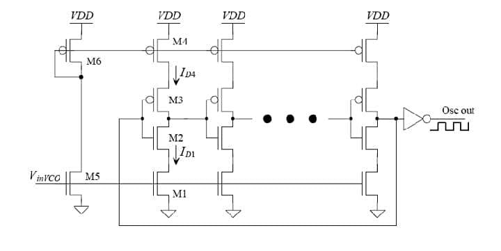
Figure 6 Current-control oscillator circuit. Image used courtesy of Bob Odhiambo
In the control of frequency and the output of the CCO’s signal after frequency comparison, which is used to make adjustments using the proportional-integral (PI) controller and can be expressed as:
CCOoutput (t) = CCOoutput (t-1) + Kp× e(t) + Ki × ∫ e(t)dt
where Kp is the proportional gain of the CCO controller, and Ki is the integral gain of the CCO controller.
This is essential in getting the modulation index to control the overall voltage output of the PV system.
By reducing harmonic distortion and flicker in the PV system, the grid synchronization technique also improves the power efficiency and quality of the grid. However, this technique is limited by factors that can reduce its effectiveness like sudden changes in the grid’s frequency and voltage.
Maximizing PV Arrays and Grid-Connected Inverters
This article has shed light on how power outputs in PV arrays and grid-connected inverters can be maximized to provide clean energy that is also reliable. Engineers can draw valuable insight into how grid-connected inverters in PV systems can be efficiently modeled using SSM and implement power control methods like P&O to ensure the power fed to the grid meets consumer demand. Below are some of the major points to note:
- The space state and transfer function models are approaches to modeling grid-connected inverters of PV systems.
- Incremental conductance, perturb and observation, and grid synchronization techniques control the synchronization and the MPPT in PV systems.
- Voltage-controlled oscillators and current-controlled oscillators are used to implement the PLL controller.
- VCO is calculated by:
\[\theta vco(s)=\frac{Kv}{s}Vc(s)\]
- The transfer function is calculated by:
\[H(s)=\frac{Vout(s)}{Vin(s)}\]