Facebook
 Google
 GitHub
 Linkedin
EMI: Understanding the Causes in Power Electronics
This article explores how electromagnetic interference affects power electronics systems, how it is caused, and how it can be prevented.
Electromagnetic interference (EMI) causes unwanted noise and reduces power quality, efficiency, and reliability in power electronics.

Image used courtesy of Adobe Stock
Electromagnetic Interference Disruption
EMI happens when an electromagnetic signal disrupts the normal operation of power electronics. This interference results from radio frequency, power lines, and electrical and electronic equipment. In power electronics, EMI causes poor performance by increasing electrical noise.
Here are the key reasons it is vital to understand electromagnetic interference in power electronics:
- Reduced power quality: EMI can cause noise, unwanted voltage spikes, and transients in power systems, reducing overall power quality, efficiency, accuracy, and performance.
- Increased noise: Higher noise levels can result from EMI and negatively impact the performance of power electronic devices.
- Interference with other devices: EMI can degrade the performance of power electronics components by creating interference with the signals.
- Reduced efficiency: Power losses and inefficiencies result from EMI, reducing overall efficiency and increasing energy consumption and costs.
Understanding electromagnetic interference in power electronics aids in designing and implementing better components to improve power quality, reduce electrical noise, and minimize interference with other systems.
Causes of Electromagnetic Interference
The causes of EMI in power electronics are complex and multifaceted. Here are some of the most common causes of EMI in power electronics.
Switching Transients
Transients and high-frequency voltage spikes, known as switching transients, are produced when power electronic systems and components are switched on and off quickly. The sudden rise and fall in current and voltage levels, parasitic inductances, and capacitances in switching circuits are just a few of the causes of transients. Switching transients produce electromagnetic interference in power electronics by emitting high-frequency electromagnetic energy.
Mathematical models are utilized to examine the switching transient behavior in power electronics. Differential equations and circuit analysis methods are the foundation. Here are a few essential equations for switching transients.
Inductor current: This equation describes the conductor’s voltage-current relationship. The rate of change in current is directly proportional to the voltage flowing across it, with the constant being the inductance. This relationship is also known as Faraday’s law of induction.

Figure 1. Circuit showing the relationship between inductor and current. Image used courtesy of Bob Odhiambo
The inductor current equation can be determined by:
\[V(t)=L\frac{di}{dt}\]
where \(\frac{di}{dt}\) is the current change rate flowing through the inductor in amperes per second.
V(t) is the voltage in volts flowing through the inductor.
L is the inductance in Henries.
Therefore, the resultant equation for the current calculation can be determined using:
\[I-\frac{1}{L}\int Vdt\]
Capacitor voltage: This equation describes the relationship between a capacitor’s voltage and current, where the voltage flowing in the capacitor is directly proportional to the current flowing through it.

Figure 2. Relationship between capacitor voltage and current. Image used courtesy of Bob Odhiambo
Capacitors store charge and filter high-frequency signals. Understanding the capacitor voltage equation is fundamental for designing these applications and is determined using:
\[\frac{dV}{dt}=\frac{I(t)}{C}\]
where \(\frac{dV}{dt}\) is the rate of change in capacitor voltage in volts per second.
I(t) is the current moving through the capacitor C.
C is the capacitance.
Differential: These equations describe the systems’ rate of change over time. They are used to design and analyze how electrical circuits and systems behave. Here are some key features that make up the differential equations in power electronics.
- Modeling circuit components such as capacitors, diodes, resistors, and inductors
- Circuit dynamic analysis includes circuits’ stability and response to changing inputs over time
- Computer simulations
- Solution methods include Laplace transform, numerical integral, and frequency domain analysis
To solve for the transient response of a simple RL circuit, the initial conditions of the parameters like inductance, capacitance, resistance, current, and source voltage are considered. Using the second-order differential linear equation, the evaluation of the transient response can be implemented using the formula:
\[L\frac{di}{dt}+Ri+\frac{1}{C}\int i\,dt=V_{S}\delta(t)\]
where \(\delta(t)\) is the Dirac delta function representing the instantaneous change in the voltage source VS at time t=0.
Common Mode Currents
Flowing in the same direction on two or more conductors, common mode currents induce a magnetic field, becoming one of the major causes of EMI.
Various sources can produce this common mode current, such as imbalanced loads, ground loops, and switching transients. The current can cause EMI issues like electromagnetic compatibility and radio frequency interference.
Several design and mitigation strategies are used to reduce the effects of common mode currents, including balanced circuits, input and output signal filtering, and low inductance components.
One of the strategies that can be used in the implementation of balancing circuits is using twisted pair impedance matching in a pair of twisted cables in which their characteristics impedance (Z0) can be evaluated using the formula:
\[Z_{0}=\sqrt\frac{1}{C}\]
where the impedance of the cable per unit length is represented by L and the capacitance per unit length of the twisted cable is represented by C.
Another approach to achieve a balanced circuit to reduce the effects of common mode currents is implementing differential signaling, which can be done by evaluating the common mode rejection ratio (CMRR) using the formula:
\[CMRR(dB)=20Log_{10}\Big(\frac{V_{differential}}{V_{common}}\Big)\]
where Vcommon represents the common mode voltage, and Vdifferential is the differential mode voltage.
When it comes to filtering the input and output signals in a balanced circuit, the common mode is used where its angular frequency and impedance are considered and can be evaluated using the formula:
\[Z_{choke}=j\omega L\]
where j represents the imaginary unit, ω represents the angular frequency, and L is the inductance.
In the filtering process of input/output signals using differential mode filters, the differential signals are allowed to pass while providing high attenuation for common mode signals.

Figure 3. Graph of the frequency response of the differential mode filter. Image used courtesy of Bob Odhiambo
Differential Mode Currents
Differential mode currents flow in opposite directions in two or more conductors. These currents do not induce significant electromagnetic fields as in common currents mode and are, therefore, not a major source of EMI.
These currents relay the desired signal between different system parts. The current is balanced and symmetrical, with the opposite current flowing in the two conductors, minimizing the circuit's electromagnetic fields and decreasing the risk of EMI.
High-Frequency Oscillations
High-frequency oscillations are fast current or voltage fluctuations that occur at high frequencies in power electronic circuits. These oscillations can cause problems such as electromagnetic interference, power loss, and reduced efficiency.
These oscillations often result from interactions between active and passive elements and parasitic elements in circuits, including inductances and stray capacitances. High-frequency oscillations can also result from fast switching of power devices and non-ideal behavior in passive components such as capacitors and inductors.
Takeaways of Electromagnetic Interference
Electromagnetic interference occurs when an electromagnetic signal hinders the normal operation of electronic components. Understanding EMI is important as it can affect power electronic systems by reducing power quality, increasing noise levels, interfering with other devices, and reducing efficiency. Common causes of EMI in power electronics include switching transients, common mode currents, and differential mode currents.