Facebook
 Google
 GitHub
 Linkedin
Power System Reliability Modeling With In-Situ MTBF Calculations
This article explores how to get started with reliability modeling using a classical theory of assessing reliability for complex systems.
Despite the complexity and technical challenges, industry interest is growing in identifying impending failures and assessing the current health of complex electrical circuits, especially for power supplies. This focus is driven by data centers and telecommunications sectors, where power supply failures pose significant risks.
For instance, according to a 2021 report by the Uptime Institute, the average cost of an unplanned data center outage is approximately $740,357, with 40 percent of the companies stating more than $1 million hourly downtime costs in the Server OS reliability survey from ITIC. Hence, seamless operations and mitigating financial impacts are urgent needs.
Traditional Approaches to Reliability Modeling
Determining the reliability and health status of electrical systems, particularly power supplies, is complex. This complexity stems from the numerous components in typical designs and the extreme conditions high-performance power supply units endure. Due to the diverse nature of these systems and their operational environments, there is no universal solution.
Potential approaches to assessing electrical circuit reliability can be divided into four primary categories, as shown in Table 1 below. Solutions vary based on deterministic or statistical modeling and whether execution is in-situ (e.g., on a power controller) or ex-situ (e.g., a cloud application).
Table 1. Different approaches to assessing electrical circuit reliability.
| Deterministic Nature | Statistic Nature | |
|---|---|---|
| Ex-situ Examples | Design Analysis: Techniques like Failure Mode and Effects Analysis (FMEA) and Fault Tree Analysis (FTA) predict potential failure points based on design schematics and operating conditions without actual physical tests. | Reliability Prediction Models: Using MTBF calculation methods, handbooks like Telcordia SR-332, MIL-HDBK-217, or proprietary models, statistical methods are applied to historical failure data and empirical formulas to estimate the Mean Time Between Failures (MTBF) or Failure In Time (FIT) rates. |
| In-situ Examples | Built-In Self-Test (BIST): These are embedded diagnostic routines that run within the system during operation to detect faults and predict failures, ensuring real-time health monitoring. | Anomaly Detection: Anomaly detection uses statistical and machine learning methods to monitor data in real-time, identifying deviations that may signal potential failures. |
To manage reliability complexities, looking further into statistical modeling and reliability prediction models is good advice.
The Bathtub Curve
A widely accepted classical approach, the bathtub curve, as shown in Figure 1, is fundamental here. It illustrates how failure rate changes over time and is described using the Weibull distribution.
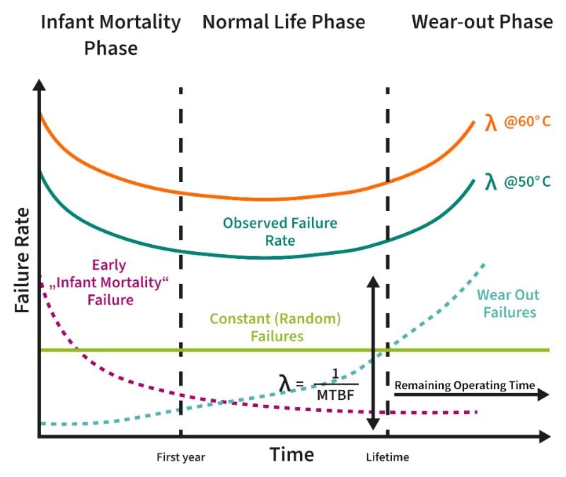
Figure 1. The bathtub curve and the contributions of different phases to the overall failure rate.
The first life cycle phase is the Infant Mortality Phase, which has a high, rapidly decreasing failure rate due to initial faulty devices. The second phase, the Normal Life Phase, sees a relatively constant failure rate as most defective devices have failed, and aging effects are minimal. The third phase, the Wear-out Phase, shows a sharp increase in failure rates due to aging and wear. The period between normal life and wear-out phases is the product's lifetime, typically designed to avoid wear-out effects.
Understanding these phases is crucial for effective reliability modeling and strategy identification.
Introducing Failure Rate Metrics
The failure rate, denoted by (Failure in Time, FIT), measures one failure per billion hours of operation, indicating the likelihood of failure within a given timeframe. The inverse of FIT, Mean Time Between Failures (MTBF) or Mean Time To Failure (MTTF), indicates the average time between failures for reparable systems (MTBF) or non-reparable systems (MTTF). This discussion uses the term MTBF (but the underlying concepts also apply to MTTF), which applies to parts or whole systems like power supplies, though methods vary. You can calculate MTBF from field tests using the formula:
$$MTBF=\frac{\text{Total Operating Time}}{\text{Number of Failures}}$$
For complex systems, consider each part's MTBF and their interactions using reliability block diagrams or fault tree analysis. Reliability handbooks can model and calculate MTBF for complex systems, which is crucial for designing durable products and identifying potential failure points before testing. This helps plan maintenance to extend product life. Let’s now explore applying MTBF calculation theory in practice.
Modeling Failure Rates With MTBF
Failures during the normal life phase are of primary interest in the field. MTBF calculation methods, as specified in reliability handbooks like Telcordia SR-332 or MIL-HDBK-217F, provide a structured approach to predict and quantify the reliability of electronic components and systems ex-situ during the design phase.
The process begins with data collection, including component specifications, operational environments, application conditions, and historical failure data. The next step involves estimating individual component failure rates (\(\lambda_{comp} \)). Handbooks provide methods to derive base failure rates (\(\lambda_{base} \)) from empirical data or manufacturer FIT reports can be consulted. For example, Infineon's FIT report for the product IPB014N06N lists a FIT rate and test conditions.
The base failure rate (\(\lambda_{base}\)) is adjusted using additional factors (\(\pi\)) that can include environmental conditions, like \(\pi_T\) for temperature, and application stresses, like \(\pi_{S}\) for electrical stress. For example, in the above graphic with the bathtub curve, two observed failure rates (blue and orange) for different application stresses are illustrated. Other factors, such as quality (\(\pi_{Q})\), may also be included.
The adjusted component failure rates are obtained by multiplying the base failure rate by the respective factors:
$$\lambda_{comp}=\lambda_{base}\pi_{T}\pi_{S}\pi_{Q}$$
The acceleration factor for temperature (\(\pi_T)\) is typically defined as:
$$\pi_{T}=e^{\frac{E_a}{k_B}(\frac{1}{T_0}-\frac{1}{T})}$$
where:
Ea is a component-specific activation energy
T is the temperature of the respective component/system
T0 is a reference temperature
kB is the Boltzmann constant.
Similarly, the electrical stress (\(\pi_S)\) is given by:
$$\pi_S=Ae^{B(s-s_0)}$$
where:
A and B usually denote component-specific shape parameters considering device-specific behavior
s is an electrical stress parameter,
s0 is a reference stress parameter.
The electrical stress parameter depends on the component as the ratio of an applied value and a rated value:
For resistors: \(s = \frac{\text{Applied Power}}{\text{Rated Power}}\)
For capacitors: \(s = \frac{\text{Applied Voltage}}{\text{Rated Voltage}}\).
The system failure rate is usually calculated once individual component failure rates are determined. For components in series, the system failure rate is the sum of all the adjusted component failure rates:
$$\lambda_{system}=\Sigma\lambda_{comp}$$
Here, additional factors, such as an environmental factor impacting all components equally, could be considered, as shown in Figure 2. For parallel configurations, additional calculations are needed. Finally, MTBF is calculated as the inverse of the total system failure rate. Figure 2 illustrates the overall approach and includes example values:
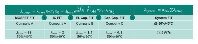
Figure 2. The calculation methods of the component failure rate and one example calculation for a system failure rate.
Following these steps, you can systematically estimate MTBF for electronic systems. However, these calculations are limited by assumptions about mission profiles and operating conditions in ex-situ scenarios. This limitation can be addressed by performing these calculations in situ.
Operating Conditions and Advantages of In-Situ Modeling
Ex-situ reliability methods' drawback is their reliance on prior assumptions like mission profiles or environmental conditions, which prevents real-time insights into a system’s health. Implementing an in-situ reliability prediction model, where calculations and monitoring occur within the system considering actual operating conditions, offers several advantages over traditional ex-situ approaches.
To address these drawbacks, Infineon has directly integrated the methodology of MTBF calculations into its power controllers. By bringing structured and standardized ex-situ reliability predictions into the in-situ environment, Infineon enables real-time monitoring and dynamic adjustment of failure rates based on actual conditions.
In an in-situ application, the system continuously monitors real-time data such as temperature, voltage, and current. This data dynamically adjusts failure rate calculations and MTBF predictions based on actual conditions. Many of these parameters are already part of the power controller's control loop (e.g., PFC control or LLC control loops), as shown in Figure 3, but they are not used for such calculations today.
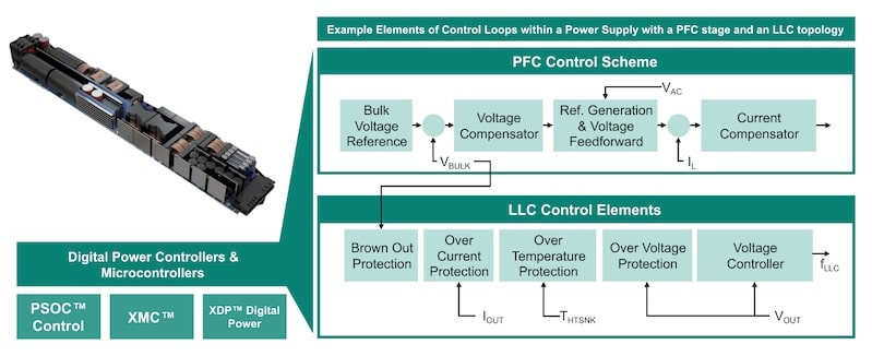
Figure 3: Control loops of a classical power supply unit with PFC and LLC, including operating parameters such as output current, temperature of the heatsink, and output voltage.
Model parameters, including base failure rates and environmental factors, are adjusted based on real-time data, allowing continuous computation of adjusted failure rates and MTBF. This provides updated reliability predictions as conditions evolve. Consequently, the system offers proactive maintenance alerts and recommendations based on calculated reliability metrics, which help compare multiple systems. Although expecting, for example, power supplies in a data center to have the same mission profile, the proposed approach allows detecting deviations from those assumptions, and respective actions can be triggered.
In-situ execution of MTBF calculation methods offers higher accuracy due to real-time data reflecting actual conditions, leading to more reliable assessments and better decisions. Continuous monitoring and dynamic calculations identify potential issues before failures occur, reducing unplanned downtime. The system adapts to varying environments, ensuring reliable predictions even under unexpected stresses.
Moreover, understanding real-time stresses optimizes operation to extend component lifespan and improve overall system reliability. This proactive maintenance approach and accurate reliability predictions can reduce emergency repairs and extend scheduled maintenance intervals, resulting in cost savings. Real-time reliability data supports enhanced decision-making for maintenance and upgrades. Continuous feedback into the design process helps engineers refine future designs based on actual field performance.
Figure 4 summarizes these benefits by illustrating the reliability boundary condition of the customer (e.g., a 3 percent maximum failure probability). Based on the actual mission profile (purple), the failure probability is calculated through in-situ MTBF modeling. Current statistical failure probability allows customers to plan maintenance, and trend analysis reveals if the system under the current mission profile risks hitting the reliability boundary earlier than initially planned (dashed purple line). In the graphic above, an average and worst-case curve is also included that shows two different assumptions on operating conditions. The sharp kink illustrates where the system, after the expected lifetime, enters the wear-out phase as described above.

Figure 4: Reliability curves are dependent on operating conditions, including the reliability requirements/boundary of a customer.
Visit Infineon for more information on power system reliability modeling, including details on how the in-situ implementation works, or Infineon’s online tool for first insights on the solution’s potential.
All images used courtesy of Infineon.