 Facebook
 Google
 GitHub
 Linkedin
How String PCS Architecture Can Improve BESS Lifetime
String-level power conversion systems increase usable lifetime energy yield in battery storage by independently managing battery strings to mitigate the effects of cell aging.
Centralized and string-level power conversion systems (PCS) for battery energy storage systems are usually compared on capital cost. On commissioning day, two PCS systems may look almost identical. The differences appear later because the cells in these systems do not age at the same rate. The weakest cell in a series string determines when discharge stops.
Rather than focusing on upfront costs, this article compares PCS architectures based on total lifetime energy yield. It tracks how cells age unevenly over time, trapping usable energy that standard cell balancing cannot recover. To quantify this gap, I will demonstrate results from a 15-year Monte Carlo simulation of a 5 MWh BESS container housing 4,992 cells across 12 strings.
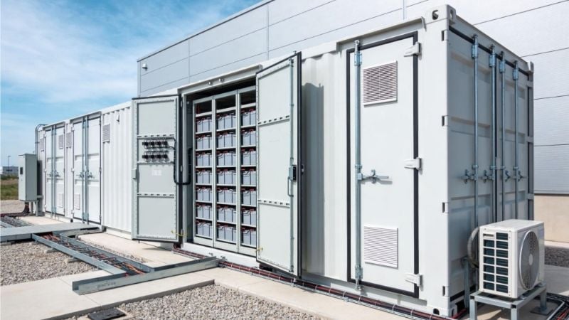
Battery energy storage system. Image used courtesy of Adobe Stock
The Problem Starts at the Cell Factory
Small tolerances in electrode coating thickness, electrolyte filling, and formation result in differences in capacity and internal resistance. In one study, across 1,100 production-fresh 3 Ah cylindrical LFP cells, the relative variation in capacity was 0.28%, and impedance was 0.72%. A follow-up study put within-batch variation at about 0.48% on a different basis, with variation between production batches higher than within a single batch. Cell OEMs sort these variances during final testing to reduce the spread and remove outliers.
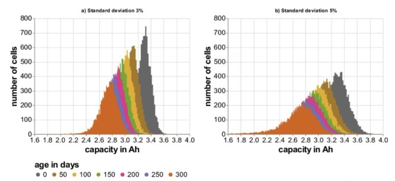
Figure 1. Variances in cells. Image used courtesy of Barbers et al.
BESS integrators then test and sort again, so cells of similar capacity and resistance end up in the same rack. On the projects I have worked on, this manual sorting has proven an efficient measure during factory production, but no such procedure exists that can be implemented on delivery day. That spread defines a 15-year weakest-cell result from the modeling.
Balancing Does Not Remove the Spread
Neither of the two balancing approaches in use removes that spread.
Passive balancing bleeds about 0.1 A through a resistor across each cell. It equalizes state of charge, not capacity, and the window is open only during a small part of the charge curve. Ampere-hours are the honest unit: bleeding off a 1% state-of-charge offset on a 314 Ah cell means removing 3.14 Ah, or 31 hours at full bleed for just 1% of capacity.
Active balancing redistributes charge between neighboring cells. It is more efficient, but it greatly increases the number of active components inside the BMS—the second-most expensive item in a BESS after the cells. Module-level BMS with active balancing are often a recurring source of in-service failures. That stops many OEMs from implementing such a strategy.
Neither corrects what the BMS cannot see: the LFP voltage curve is flat across the middle, so SOC is re-anchored only near the top and bottom, and an estimate off by a few percent mis-targets the balancing itself.
What ‘String PCS’ Means and Why the Weakest Cell Decides the Whole Block
The term "string PCS" is used loosely, and what matters is not the label but the smallest section that can be dispatched, tripped, and maintained independently. Here, that section is one battery string behind a dedicated AC PCS, matching the 230 kW inverters for current 5 MWh systems, 12 per container. Each battery string has a separate PCS. A central PCS can have independent DC inputs, yet one DC input generally serves a full 5 MWh container.
That smallest independent section sets the stop rule. A BMS ends discharge on the lowest cell voltage or the string voltage; dispersion trips the first, so the usable window is set by the weakest cell sharing it.
Under a central PCS, the population is 4,992 cells (416S12P), with paralleling occurring at the string level on the DC bus, each string maintaining its own series chain of 416 cells. Under string PCS, each section stops on the weakest of its own 416 cells (416S1P). The difference is energy left unused in the healthier strings.
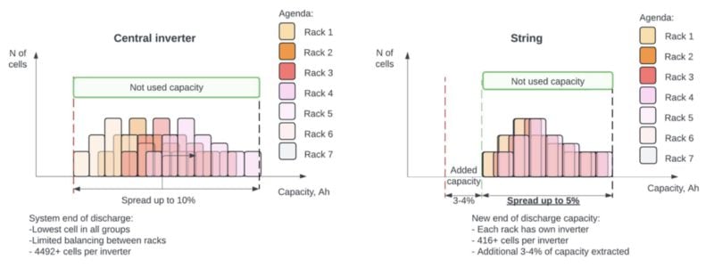
Figure 2. Inverter vs. string.
What Independent Control Changes
Independent string control can allocate less current to a weak or hot section and work each section against its own limits. It does not reverse chemical degradation or guarantee longer cell life, but it can increase the energy a fleet delivers as cells age unevenly.
Table 1. Monte Carlo model inputs.
| Input | Value |
| Container | 12 strings × 416 series cells = 4,992 cells; 314 Ah cell; 5.016 MWh nominal |
| Horizon | 15 years, 240 steps of 22.8125 days per step |
| Duty | one 80% depth-of-discharge(DOD) cycle per day |
| Degradation | 2.2% mean annual fade + cycle-loss assumptions from vendor curves |
| σ initial capacity | 0.5%; around what is measured on 3 Ah cylindrical LFP cells in research. |
| σ aging rate | 5%, value mentioned in research papers |
| σ duty share | 1%, estimated string-to-string drift with impedance and state-of-health (SOH) mismatch on a common DC bus |
| Number of independent simulations | 20 |
| Total computation operations per simulation |
24,000,000 per container |
What the Simulation Found
The simulation model constants were calibrated against representative degradation curves from leading Tier 1 vendors for operating profiles of 0.5, 1, and 2 cycles per day. These reference curves reflect the real-world calendar and cycle-aging behavior of commercially available LFP cells.
The underlying degradation curves are based on extensive physical testing of thousands of cells over thousands of charge–discharge cycles, providing an empirical foundation for predicting long-term cell performance.
String's advantage in lifetime delivered energy, to retirement at 70% SOH, is 6.25% mean, 6.3% P50, and 1.2% P90, with a much wider dispersion. That gap is largely commercial: warranties are written on SOH, so the model is the central case as retired-in-whole at 70%, while strings above it keep working.
The numbers have limits. Because the simulation stopped the entire central-PCS container on its single weakest cell—without allowing controls to isolate weak strings via contactors—this 6.25% gap represents a theoretical upper limit for String PCS's advantage over an unmanaged central architecture.
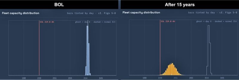
Figure 3. Distribution of cell capacity across the fleet when new and after 15 years.
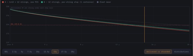
Figure 4. Deliverable Ah per string under each stop rule. The display axis runs to 20 years; the Monte Carlo horizon is 15 years.
In analyzing two mean capacities, the percentiles compare energy in one year-15 discharge, round by round, with a mean of +2.12%.
Table 2. Mean 15-year container capacity, central versus string stop rule.
| Metric | Central PCS | String PCS | Difference |
| Mean 15-year container capacity, 20 rounds | 3.36 MWh | 3.43 MWh | +2.1% |
Both values reflect the remaining container capacity relative to a nominal 5.016 MWh rating (about 67% and 68%). Consequently, both fall below the 70% state-of-health retirement line used in the analysis. That figure is capacity left on a fixed date; the lifetime figure counts energy delivered before retirement. Both stop rules run on the same draw, so the cells are identical: the 2.1% is additional energy that string inverters allow.
Upon examining more details of each of the 20 simulations, a more interesting picture emerges.

.jpg)
Figure 5. ΔE per discharge at year 15, per container, 20 draws (top). Lifetime ΔE per container, fleets retired at 70% EOL, 20 draws (bottom).
P50 +2.08%, P90 +1.28%. P90 is the exceedance level, beaten in 90% of draws; with 20 rounds, the second-worst, so read it as indicative.
It means even in most conservative cases, string inverters show additional capacity.
Additionally, lifetime capacity also changes in String and Central inverter scenarios.
What This Means
Dispersion is the normal condition of an aging series-parallel fleet, and it widens. The architectural question is what the control system is permitted to do about it. A weakest-cell stop rule across 4,992 cells discards more than the same rule does across 416 cells.
In real-life applications, mathematically we can expect string inverters around 2% higher capacity after 15 years and around 6% more energy delivered before EOL in the average case, with P90 estimates also showing the advantage of string inverters.
None of this says string always wins, but mathematically this approach looks more favorable. A central PCS with genuinely independent DC control and several DC inputs connecting to different containers recovers part of the spread.
Figures and tables used courtesy of Sergey Syrvachev.