Facebook
 Google
 GitHub
 Linkedin
Optical Electric Field Sensor for High Voltage Equipment Diagnostics
This article highlights Kapteos SAS New Products such as Optical Electric Field Sensor used for Electrical Diagnostics of High Voltage Equipments.
Power transmission, power plants, or any high power electronics systems involve high voltage (HV) devices which have to be controlled or even monitored over a significant amount of time.
To ensure the reliability of the power grid and the power quality of the supplied energy, the electric and dielectric behavior of medium voltage (MV) and high voltage (HV) devices have to be carefully assessed. For that purpose, the energized cables behavior, the insulator properties of insulators, the power semiconductors features shall be investigated.
Sensing Techniques
Today the measurements required for this investigation are essentially performed using voltage transformers such as resistive, capacitive or inductive dividers in case of contact measurement or with metallic antennas for contactless field measurement. Such sensing techniques are limited firstly by the setting up constraints (e.g., required galvanic connection to the device under test) and secondly by their inherent poor spatial resolution and induced interference.
The aim of this article is to demonstrate the advantages of pigtailed optical sensors to perform electric (E) field characterization in the vicinity of MV and HV electrical devices. The probe used for this E-field measurement presents the following characteristics:
- Measurement of E-Field magnitude and phase of each vector component
- High electrical insulation (fully dielectric pigtailed probe)
- Spatial resolution down to 1 mm
- Fully independent of magnetic field and current (up to MA)
- Absolute field strength measurement thanks to easy probe calibration (uncertainty weaker than 1 dB)
- Time domain measurement down to sub-nanosecond
- Frequency bandwidth exceeding several GHz
- Compact probe
- High dynamic range (up to air breakdown field)
- Fully compatible with various environments (gases, liquids like oils, temperature and hygrometry variations)
- Single point measurement or multidimensional mapping using rotation or translation stages

Figure 1: Electro-optic probe and associated optoelectronic converter.
Electro-Optic Probe
The optical probe is seen in the foreground of Figure 1 and is here mounted on an HV compliant articulated holder. The probe consists of a dielectric optical modulator and acts as a linear transducer between the E-field component to be measured and the modulation of a laser beam. Its transverse dimension does not exceed 5 mm and its sheath permittivity is εr = 4.
This probe is plugged in an optoelectronic converter thanks to optical fibers (see the background in Figure 1). This converter includes both a low noise laser feeding the probe and an optoelectronic subsystem delivering an electric signal directly proportional to the E field. The setup ensures a real-time measurement of the E field over a frequency range spreading from some 10 Hz up to several 10 GHz. The link between the analog output voltage Vout and the actual field value Eactual is given by the antenna factor AF:
Eactual = AF x Vout
AF is given in m-1. Its numerical value is defined by the calibration of the probe. Such calibration remains valuable over a dynamic range greater than 120 dB covering field values from less than 1 V/m up to more than 1 MV/m. The air breakdown field can even be measured. The AF of the whole system is monitored all along the measurements. The output signal can be acquired using an oscilloscope for time domain measurement or a spectrum analyzer for frequency domain measurement.
Representations for Analysis
Voltage and Field Measurements
The first example is dedicated to contactless diagnostic of a 100 kV hollow insulator using the same optical probe. The applied voltage is acquired and synchronized with the radial field measurement. Two configurations are compared.
The insulator is firstly characterized in nominal conditions. The voltage and field measurements correspond to the blue curves of Figure 2. Then, a defect is simulated using a high resistor placed inside the hollow insulator. The defect consists of a 10 GΩ, 30 cm long resistor.
The measurements correspond to the red curves of Figure 2. One can notice that the measured voltage does not exhibit any relevant signature of the defect.

Figure 2: Voltage (top) and electric field (bottom) measurements. Blue color corresponds to the nominal behavior of the insulator. Red color corresponds to the insulator with a defect.
Thus, voltage analysis can definitely not be used as a valuable mean for diagnostics. On the contrary, the E-field temporal waveform is dramatically modified by the inner defect: both magnitude and phase are heavily modified. Indeed, the defect induces a huge phase shift of 130° and an enhancement of 50% of the magnitude.
E Field Mapping Over a Laminated Busbar
The second example illustrates the E field mapping over a laminated busbar used in power electronics. The probe is mounted on a Cartesian robot and its position is acquired simultaneously with the field value of the component which is normal to the plane of the laminated busbar. E field mapping corresponds to a near field measurement as the probe is located less than 5 mm from the busbar surface. The spatial resolution of the measurement is 0.5 mm.

Figure 3: Measurement - 2D field mapping of the normal component in the vicinity of a laminated busbar. Top: dry condition. Bottom: wet condition.
The result is presented in Figure 3 for two different conditions: 1) dry and stabilized thermal conditions, 2) moisture and water saturated air inducing liquid droplet on the busbar.
The difference between the two mappings are significant with an increase of the field heterogeneity. As a matter of fact the field vanished down to 0 V/m in the bottom left and increased by a factor 2 on the right of the mapping. The authors point out that this result could not be assessed by numerical simulations.
E-field Characterization in the Vicinity of MV and HV Devices
The last example describes the E-field characterization in the vicinity of MV and HV devices: analysis of the field radiated by seven different 25 kV cables. This characterization concerns the apparition of partial discharges (PD) due to corrosion or contamination which can be significant for ageing cables in outdoor conditions.
This kind of analysis is usually performed a posteriori with a visual inspection of the disassembled cable. We here propose to characterize the E-field in the vicinity of the cable to assess its behavior under voltage.
The cables are here fed by a 50 Hz signal provided by a transformer delivering a voltage from 0.2 kVrms to 25 kVrms. The temporal waveform of the radial E-field is measured and acquired with a sampling rate of 20 MS/s for each cable and for each voltage value.
The data are then analyzed (total harmonic distortion, linearity with applied voltage, residue versus pure 50 Hz signal, wavelet transform ...).
Multidimensional Representation
We here propose a multidimensional representation to compare the behavior of the 7 cables under test. In Figure 4, the first axis represents the voltage threshold for the apparition of PD (PD thresh-old [kV]). The second axis is the overvoltage magnitude (O.V. [kV]) linked to PD. Finally, the last axis represents a phenomenological non-linearity factor ζ giving the deviation to linearity when PD appear. The characterizations of the 7 cables under test are synthesized as dots on the 3D representation given in Figure 4.

Figure 4: Multidimensional analysis of partial discharges on several 25 kV cables.
The red dot, localized at the origin, corresponds to the reference cable (new cable without aging). For this reference cable, the voltage of PD appearance is the highest (15 kV), the non-linearity factor ζ is the lowest (0.5) and the overvoltage value is moderate (12 kV).
All other cables present different aging factors. Brown, green, and yellow dots, which are far from the origin, are symptomatic of highly degraded cables that should be replaced.
Conclusion
We demonstrate via a few examples the relevance of electrooptic technology for measuring E fields. This technology is particularly adapted for near field measurements, even under HV conditions, from few tens of Hz to several tens of GHz. The electrooptic technology is of major interest for analysis of power electronics modules using SiC technology or for HV components. It is very helpful for engineers and technicians to analyze and to understand the phenomena of fatigue, ageing, contamination, and corrosion as the E field appears to possess relevant and distinctive signatures of these phenomena.
About the Author
Gwenaël Gaborit is an Associate Professor at the Université Savoie Mont Blanc and the CSO at Kapteos.
Lionel Duvillaret is the Chief Executive Officer of Kapteos. His expertise includes optoelectronics, optical physics, and electromagnets.