How To Build a Battery Model Using Fuel Gauging—Part I

With many modern devices and systems transitioning to cordless operation, their power delivery changes from mains to battery power. This requires that information about the battery's state be readily available to the system for optimal performance and efficient operation.

 

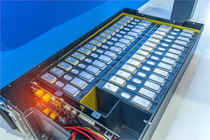
Image used courtesy of Adobe Stock

 

What Is Fuel Gauging?

Fuel gauging is a set of techniques that can provide accurate information about the battery’s health, state of charge, and other critical system parameters. Inaccurate fuel gauging can result in unexpected device shutdowns or subpar performance, causing inconvenience, damage, and safety hazards.

Mains power gives a steady, regulated line voltage and current as demanded by the device or system. Unlike mains power, battery power and capacity fluctuate due to temperature, usage pattern, and battery age. Consequently, fuel gauging ensures the device has adequate power to perform optimally and prevents overcharging or over-discharging, which can adversely affect lifespan.

Fuel gauging can be implemented through hardware-based systems or software-based algorithms that track battery performance and provide precise readings of the remaining capacity. Some devices may estimate battery life based on usage patterns and history.

The simplest electrical battery model is, as shown in Figure 1, a voltage source in series with an internal resistance. This model represents the idealized behavior of a battery as a constant voltage source, and it can maintain a fixed potential difference across its terminals if it has a charge. This is connected to an internal resistance that models the losses due to the battery's internal chemical and physical processes.

 

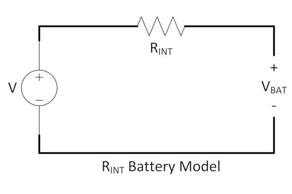
Figure 1. R_INT battery model. Image used courtesy of Qorvo

 

In this model, the voltage source has a value that is the difference between the battery's positive and negative terminals when no current is flowing. This is electromotive force (EMF). In fuel gauging, it is more commonly called open circuit voltage (OCV).

\[V_{i=0}=OCV\,or\,V=OCV\]

The internal resistor represents the battery's internal losses and resistance to current flow, which cause the voltage to drop when current flows through the battery.

The battery is also defined to have a chemical energy capacity denoted by Q. This is the energy it can deliver from being fully charged to fully discharged. The units for the capacity are Ah(Amp-hr). When fully charged, the battery has a state of charge (SOC) of 100%. The terminal voltage of the battery under fully charged conditions is denoted by V_(SOC=100). When fully discharged, it has a state of charge of 0%. The terminal voltage of a fully discharged battery is denoted by V_(SOC=0).

When connected to an external circuit, current flows through the circuit; the voltage across the battery's terminals drops across the internal resistance, as shown in Figure 2. This voltage drop can be modeled using Ohm's Law—that is, the voltage drop is proportional to the current and the internal resistance.

 

Figure 2. R_INT battery model when connected to a load. Image used courtesy of Qorvo

 

If Z = V_BAT, then the equations for this model can therefore be given as

\[V_{BAT}(t)=V(t)-i(t)R_{\,INT}\,and\]

\[Q=\int\limits^{t(soc=0)}_{t(soc=100)}i(t)dt\]

If the SOC is a ratio of the remaining capacity of a partially discharged battery to a fully charged battery, then

\[SOC=\frac{Q_{t}}{Q}\times100\%\]

The battery’s OCV can be characterized at each percentage point of the state of charge. This fundamental concept finds much use in fuel-gauging algorithms used by modern battery management systems.

However, the R_INT model has limitations: 

State of charge voltage dependency: Batteries are not ideal voltage sources; their terminal voltage depends on loading conditions and the state of charge. The terminal voltage can vary non-linearly with load, exhibiting hysteresis as loading changes, which a simple voltage source model cannot represent.

Temperature dependency: The energy stored in a battery is released due to internal chemical reactions. These reactions produce heat, changing the rate of the chemical processes. Therefore, the internal resistance of a battery varies with temperature, which can affect its performance and discharge characteristics. The simple model assumes a fixed internal resistance, which does not account for the temperature dependency of real batteries.

Self-discharge and aging: Batteries also lose charge over time due to self-discharge. They can also lose capacity as they age and have many charge-discharge cycles. Both these characteristics can affect the available capacity. The ratio of nominal available capacity at any time (Q_t) over the nominal available capacity of an unused new battery (Q_t=0) is the state of health (SOH).

\[SOH=\frac{Q_{t}}{Q_{t=0}}\]

The simple R_INT model can be improved by considering a Thevenin battery model with a single RC branch. Such a model is shown in Figure 3.

 

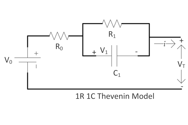
Figure 3. 1R 1C Thevenin Model. Image used courtesy of Qorvo

 

The Thevenin model adds an RC loop to the internal resistance denoted by R₀, where R₀ models the battery’s electrolyte and terminal resistances (ohmic). The resistance (R₁) and capacitance (C₁) denote the polarization. With R₁ in parallel with C₁, this representation can better model the battery's nonlinear polarization response in response to charging or discharging conditions.

Polarization is a process by which charge separation occurs inside the battery, causing a net non-zero potential. This potential opposes the external voltage, thereby limiting the battery's efficiency. 

As the battery approaches full charge with external charging, this potential approaches the externally applied voltage. This can be viewed as increasing internal resistance to an applied charge. The net effect is a reduced charging current as the battery is charged.

During discharge as the capacitor C₁ is discharged, the voltage across the capacitor also drops. This reduces the terminal voltage and in combination with the internal resistance R₀ and the polarization resistance R₁ models a reduced ability to deliver current.

The voltage equations governing this model are

\[V_{T}=V_{0}-iR_{0}-V_{1}\]

where i is the load current and V1 is the drop across the RC loop and

\[V^{'}_{1}=\frac{V_{1}}{R_{1}C_{1}}+\frac{i}{C_{1}}\]

The limitations of the 1R1C Thevenin model are:

1. It assumes a single time constant across both charge and discharge. This is inaccurate as the voltage across the battery depends on a changing internal resistance and capacitance.

2. The model does not compensate for changes in resistance at both the end of charge and the end of discharge.

3. Resistance and capacitance temperature dependence are not considered.

4. In addition to polarization, charge diffusion is due to electrolytic migration in a battery. This results in the battery capacity at any time Q_t being a function of the state of charge (SOC). The 1R1C does not model this.

Improving the 1R1C model by adding another RC loop to accommodate the diffusion behavior, different polarization rates, and temperature dependence is possible. This model is shown in Figure 4. It is called the 2R2C model or the dual polarization model.

 

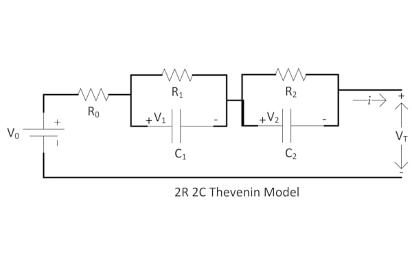
Figure 4. 2R2C Thevenin Model. Image used courtesy of Qorvo

 

Akin to the 1R1C model, in the 2R2C model, R₀ serves as the ohmic resistance, while R₁ and C₁ model the polarization resistance and capacitance. The added R₂ and C₂ components help model the voltage transient behavior and charge diffusion during charging and discharging. Because of this, the R₁ and C₁ values can be better tailored to represent the charge separation and gradient in charge across the double-layer capacitor that develops within the battery.

The equations for this model are where V1 and V2 are voltages across R₁C₁ and R₂C₂

\[V^{'}_{1}=-\frac{V_{1}}{R_{1}C_{1}}+\frac{i}{C_{1}}\]

\[V^{'}_{2}=-\frac{V_{2}}{R_{2}C_{2}}+\frac{i}{C_{2}}\]

The time domain equation for this model is derived as

\[V_{T}=V_{0}+iR_{1}\Bigg(1-e^{\frac{-t}{\tau_{1}}}\Bigg)+iR_{2}(1-e^{\frac{-t}{\tau_{2}}})\]

where

\[\tau_{1}=R_{1}C_{1}\,and\,\tau_{2}=R_{2}C_{2}\,and\,\tau_{1}>\tau_{2}\]

These time domain equations can be solved using Laplace transforms. Once solved, a further transformation into difference equations can be applied to develop linear coefficients across the entire charge-discharge cycle of the battery.

With experimental data obtained from cycling, it is possible to model the following:

• R₁, the electrolyte resistance from ionic concentration and its change due to temperature
• R₂, the electrode resistance, modeling its thermal coefficients and its change across temperature
• C₁, the double layer capacitance due to polarization at the electrode-electrolyte interface and its temperature dependence
• C₂, the diffusion capacitance due to the concentration gradient that occurs from the movement of charge across the battery

This model provides a good foundation for developing a gauging method using the equivalent circuit and a lookup table. 

The second part in this series will focus on developing a full gauging solution using coulomb counting and a lookup table. Such a solution enables greater accuracy across the discharge profile, allowing for better capacity prediction. Further optimizations for temperature and aging can also be implemented by modeling the rate of change of the battery’s inherent characteristics.