Designing Electronics to Pass the EMC Test Part 3

In Part 1, we learned one of the mechanisms that lead to CE (Conductive Emission). In Part 2, we saw how understanding the emission path can help us find solutions during the EMC test.

Sometimes the answer is not intuitive, and experience plays a significant role. EMC requires a designer/engineer to see his or her design not just from a time domain but also from a frequency domain. We’ve seen that modifying the return path can sometimes improve the CE. Part 3 will start with a real-life example, simulating and evaluating the CE using LTSpice.

We will start to see how to simulate the CE using LT Spice (or similar tools). In Part 1, we learned that the EUT (Equipment Under Test) is connected to the main or power supply using a LISN (Line Impedance Stable Network). We have learned that a LISN can be seen as a low pass filter that normalizes the power impedances (so the same measurements can be done by different EMC houses). We will learn how to model a LISN using LTSpice, how to model a power cable and how to estimate Cp (the capacitance between the EUT and the vertical/ horizontal plate in the EMC house).

I’m assuming that you are already familiar with LTSpice. If not, then go to www.analog.com and download LTSpice.

 

A Spice Model for a LISN

As discussed previously, a LISN in simplistic terms can be seen as a low pass filter for our EUT and normalizes the impedance seen from the input power terminal of our EUT. The LISN schematic drawing is often shown in the relative EMC standard. Therefore, to create a spice model for our EUT, the best thing to do is check the LISN model from the standard.

For this discussion, let’s assume we are using a “standard” 50 uH LISN from the MIL-STD 461 (see figure 1 below). The first thing we should notice is that the spectrum analyzer needs to make two measurements, one for the “positive” power input and the second for the “negative” input pin (if we are connected to the Live and Neutral we need to repeat the measurements between Live and then Neutral and).

Please notice the measurements always reference the earth (see figure 1).

Now we can call Vc the common mode voltage on V1 and V2 (referred to the EARTH) and Vd the differential voltage on V1 and V2. and we can state by definition of common mode voltage and differential mode voltage that

•Vc = (V1+V2)/2

•Vd = (V1-V2)/2

The above equation will be used later when we will start to do some simulations.

 

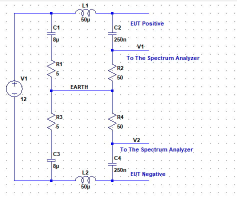
Figure 1. Typical “50 uHenry” LISN. Image used courtesy of Francesco Poderico

 

We are now in the position to estimate the common mode voltage and differential mode voltage of any circuits, given the following hypothesis:

1. We know the parasitic capacitance between our EUT and the earth plate Cp (we have seen this in Part 1, do you remember?)

2. We don’t have emissions due to a lousy layout (we will see this later in this series, how the creation of a loop antenna creates common mode noise)

3. We don’t have emissions due to the lack of bulk capacitors.

 

Estimation of Cp

Cp is usually between 20 pF to 200 pF. In my design, I estimate Cp as follows: I want to estimate the parasitic capacitance between my EUT and an infinite plane 80 cm (we have learned this in Part 1, you need to check your setup from the standards) apart from my EUT in the air. I can use the formula C= A/s where is the dielectric constant of the air, s = 80 cm and A = 10 * x * y ( x,y = PCB dimensions); so, for example, for a PCB of 100 cm x 50 cm Cp is around 110 pF.

 

Impedance Estimation of the Power Cord

We need to add a model for the power cable to the LISN model we have just seen. The model can be as simple as an Inductor in series with a small resistor (I’m ignoring the capacitance parasitic of the cable since this helps us filter both Vc and Vd).

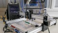
To estimate the parasitic inductance of the cable, the most accurate way to do this is to check in the cable datasheet the inductance per meter of the cable. If this information is unavailable, another way is to measure with an LCR meter, as shown in the picture below.

 

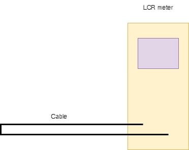
Figure 2. With the above setup, we can measure the cable inductance with an LCR meter. Image used courtesy of Francesco Poderico

 

Once we have estimated the cable inductance, we can add this to our spice model. Let’s say our cable has an inductance of 1 H and a series resistor of 0.01 ohms. Our spice model becomes:

 

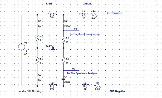
Figure 3. Spice model with LISN + power cable model. Image used courtesy of Francesco Poderico

 

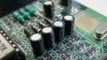
Capacitor Models

An ideal capacitor has an impedance that decreases with the frequency with a relation that follows this law: Zc = 1/C. Unfortunately, an ideal capacitor doesn’t exist, so we must add at least two parasitic components. 

1. The ESR (Equivalent Series Resistor) 

2. The ESL (Equivalent Series Inductance)

3. Rp (capacitor parallel resistor, we can neglect this for this analysis)

The ESR and ESL are usually available in the capacitor datasheet. However, if they are not, measure them using an LCR meter.

Now we are ready for some interesting simulations! Stay tuned for Part 4.

Here, we have learned how to model a LISN, how to estimate Cp, how to assess the power cable inductance, and that it is essential to use a suitable model for all the capacitors involved in the switching. In the next part, we will see this with some examples.

 

Feature image used courtesy of Pixabay