Examining Alternative Battery Models—Part II

Part 1 of this series discussed the need for fuel gauging, examined the setup of an equivalent circuit model to represent the battery, and discussed approaches to and shortcomings of this method.

 

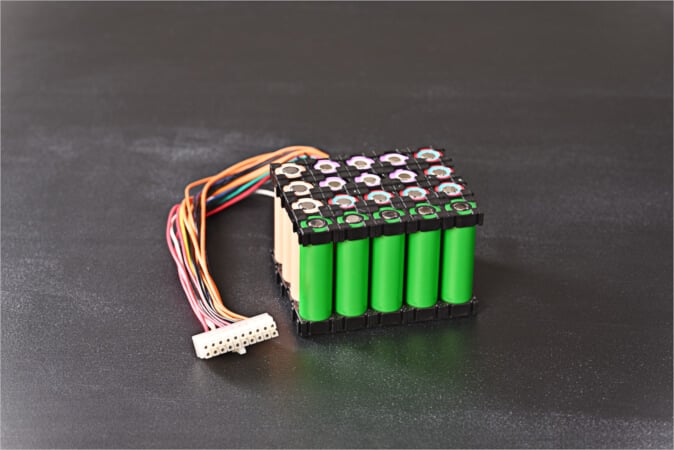
Image used courtesy of Adobe Stock

 

Part 2 examines why alternative approaches, though used in research, have yet to be commercially adopted including:

• Electrochemical
• Extended Kalman filter
• Physical charge diffusion

 

The Electrochemical Model

The electrochemical model depends on charge mobility based on the Nernst equation. This calculates the direction of a redox reaction. It provides the overpotential based on temperature and other dynamic factors. 

Taking the example of a lithium cobalt battery, if we defined the following:

\(E_{a}\) = the potential at the anode under non-standard conditions

\(E^{°}_{a}\) = the standard potential at the anode

R = the gas constant

T = the temperature in Kelvin

F = the Faraday constant

Along with \([Li^{^{+}}]_{e}\) as the Li+ ionic concentration in the electrolyte

\([C_{6}]_{_{_{_{_{S}}}}}\) and \([LiC_{6}]_{_{_{_{_{S}}}}}\) as the concentrations of C₆ and LiC₆ in the solid phase in the anode then

\[E_{a}=E_{a}^{°}+\frac{RT}{F}\cdot ln\frac{[Li^{^{+}}]_{e}[C_{6}]_{_{_{_{_{S}}}}}}{[LiC_{6}]_{_{_{_{_{S}}}}}}\]

Similarly, defining:

\(E_{c}\) = the potential at the cathode under non-standard conditions

\(E_{c}^{°}\) = the standard potential at the cathode

\([CoO_{2}]_{_{_{_{_{S^{^{^{'}}}}}}}}\) = the concentration of CoO₂ in the solid phase in the cathode

\([LiCoO_{2}]_{_{_{_{_{S^{^{^{'}}}}}}}}\) = the concentration of LiCoO₂ in the solid phase in the cathode then

\[E_{c}=E_{c}^{°}+\frac{RT}{F}\cdot ln\frac{[Li^{^{+}}]_{e}[CoO_{2}]_{_{_{_{_{S^{^{^{'}}}}}}}}}{[LiCoO_{2}]_{_{_{_{_{S^{^{^{'}}}}}}}}}\]

The effective voltage of the battery can be expressed by summing the half equations from the anode and cathode as follows

\[\Delta E=E_{c}^{°}-E_{a}^{°}+\frac{RT}{F}\cdot ln\frac{[LiC_{6}]_{_{_{_{_{S^{^{^{}}}}}}}}[LiCoO_{2}]_{_{_{_{_{S^{^{^{'}}}}}}}}}{[C_{6}]_{_{_{_{_{S^{^{^{}}}}}}}}[LiCoO_{2}]_{_{_{_{_{S^{^{^{'}}}}}}}}}\]

While the battery is used, the anodic concentration [LiC₆]_s decreases in the solid phase and the concentration of [C₆]_s increases. At the cathode, the concentration of CoO₂ in the solid phase of the cathode [CoO₂]_s′ decreases, and the concentration of LiCoO₂ in the solid phase of the cathode, [LiCoO₂]_s′ increases. Therefore, during discharge, the voltage of the battery decreases. Similar equations can be written for chemistries such as LFP, LMO, LSB, LTO, and others.

While this is a simple example of how the chemical reaction generates an electric potential, it does not model the secondary effects of battery construction and usage on the concentration of the ions. Like the anode, cathode, and electrolyte, lithium-ion batteries also contain binders, conductive additives, stabilizers, and solvents. As the battery ages and undergoes several charge-discharge cycles, these materials undergo physical degradation, resulting in material decomposition, disordering, plating, and undesirable interactions at the anode and cathode. It also affects the membrane permeability of lithium ions due to changes in the size of the particulate matter. This physical disruption results in decreased absorption rates of the ions at the anode. Due to partial absorption, metallic dendrites form on the anode surface by accumulation. This results in a loss of active lithium in the cell and large differentials in the localized electrode potential. 

In fuel gauging, it is imperative to continuously monitor the state of charge, state of health, and other parameters through a single charge-discharge cycle. These must be monitored throughout the lifetime of the battery pack. This implies that the measurements required for the monitoring must be continuously collected at a rate that enables a reasonable and usable level of accuracy. So, the calculations for a single iteration of the desired parameters should be fast enough to be usable when the value is reported. 

The calculations to model these variables are complex and require extensive computing power to accommodate different real-life rates. This is easy to do without power limits, but power is limited in a battery application. So, the model needs to be extensively simplified to accommodate the low power requirements at the cost of accuracy. So, while it finds use for research purposes, it is not a viable route to model all the discharge characteristics in practical applications.

 

The Extended Kalman Filter Model

The Kalman filter, often called linear quadratic estimation (LQE), is used extensively in control systems and statistics for predicting future values. The method uses a series of unfiltered measurements taken over time and uses their stochastic properties to derive an accuracy better than a single measurement. The basic steps of a Kalman filter are shown in Figure 1.

 

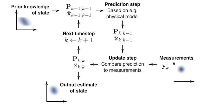
Figure 1. The basic steps of a Kalman Filter. Image used courtesy of Wikipedia, Petteri Aimonen (Creative Commons License)

 

Fundamentally, in a Kalman filter, all noise in the measurements of the independent input parameters is assumed to be Gaussian with a zero mean. This assumption implements a two-step process, as shown in Figure 1.

Here, based on the prior knowledge of the state of the system, the Kalman filter makes a prediction. This prediction contains the value and measurement’s confidence level, which can be interpreted as uncertainty. Based on the measured variables fed into the system, the prediction is updated using the method of weighted averages. The higher the confidence in the measurement, the higher the weight assigned. Now, applying the prediction and update steps recursively, any future action only requires the updated measurement from the inputs and the previously obtained confidence levels, eliminating the need for a detailed historical log of the inputs.

However, in the case of rechargeable batteries, the potential generated depends not only on the reaction rate but also on the concentration of the ions, which exhibits an exponential dependency. Therefore, the problem becomes non-linear. This model of a Kalman filter that can incorporate non-linear inputs is called the Extended Kalman Filter or the EKF.

The EKF adapts the linear quadratic estimation provided by the regular Kalman filtering for use in nonlinear systems. Here, the input and state space variables are assumed to be nonlinear and differentiable. If we defined the following:

X_k = state of the system at time interval k

X_k-1 = state of the system at time interval k-1

Z_k = the measurement or observation of the true state of the system X_k  at time interval k

u_k = the control vector of the system at time interval k

w_k = the process noise of the system at time interval k

F_k = the state-transition model

H_k = the observation model

v_k = the observation noise

Then

\[x_{k}=f\Big(x_{k-1},u_{k}\Big)+w_{k}\]

\[z_{k}=h\Big(x_{k}\Big)+v_{k}\]

For simplicity, if we used the 1R1C model defined in the previous article illustrated in Figure 2.

 

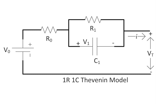
Figure 2. 1R 1C Thevenin Model. Image used courtesy of Qorvo

 

The voltage equations for the circuit are

The voltage equations governing this model are

\[V_{T}=V_{0}-iR_{0}-V_{1}\]

where i is the load current V1 is the drop across the RC loop and

\[V^{'}_{1}=-\frac{V_{1}}{R_{1}C_{1}}+\frac{i}{C_{1}}\]

If we define 

C = Rated battery capacity

SOC_t = State of charge at any time t

μ_k = The temperature correction factor in percentage change in capacity per deg K

Then, the SOC at time t can be calculated as

\[SOC_{t}=SOC_{t0}+\frac{\int\limits^{t}_{t0}\mu_{k}i(\tau)d\tau}{C}\]

Typically, in battery management systems, the initial state t0 is defined by the open circuit voltage (OCV) measured at time t0 without a load on the system. So, the function becomes

\[SOC_{t}=SOC(OCV)+\frac{\int\limits^{t}_{t0}\mu_{k}i(\tau)d\tau}{C}\] 

where the OCV is the open circuit voltage for the appropriate state of charge measurement under standard conditions.

So, having obtained the Kalman model as well as the control space vectors for the system, if we define

vk= the observed value of noise at the moment k

xk-1= the state space process value of noise at moment k-1

ΔT= the delta step size

The state space model to be solved can be written as

\[\Big[SOC_{k}-V_{T,k}\Big]=\Bigg[100e^{\frac{-\Delta T}{R_{1}C_{1}}}\Bigg]\Big[SOC_{k-1}-V_{T,k-1}\Big]-\Bigg[\frac{\Delta T}{C}(1-e^{\frac{-\Delta T}{R_{1}C_{1}}})R_{1}\Bigg]I_{k-1}+\]

And 

\[V_{T,k}=OCV(SOC_{k})-V_{1}-R_{0}I_{k}+v_{k}\]

The series expansion method can be employed to solve these sets of non-linear equations. The solution provides the next estimated state space value. This predicted value is compared against the observed change in the state of charge. The variance between the two values calculates the Kalman filter gain. This gain is used to adjust the weights in the feedback loop for the observed vs. the predicted values to tune the filter output and improve its accuracy. Therefore, the prediction correction mechanism employed by the Kalman filter provides a very close approximation for known types of loads and improves this model’s accuracy over time.

The Kalman filter has been developed for a 1R1C model in the above example. In Part 1, the shortcomings of the 1R1C model were explained. While mitigated to a certain extent by the inherent feedback loop in the Kalman filter, these are also present in the state-space-based model. Using a 2R2C model would increase the time complexity and increase computational processing capability requirements. In addition, the rate dependencies of the time series prediction can provide false high confidence levels in estimation. This can lead to the need for corrective factors, affecting prediction accuracy in transients or with a spiky load. If the variances are above an acceptable threshold, further time series averaging of the independent inputs will be required; this increases the time for obtaining the next state space estimate. Therefore, the EKF model, while used in research, is generally not found in lower-power battery management system (BMS) applications due to model-based and computational limitations.

 

The Physical Charge Diffusion Model

The final model discussed in this article is the physical charge diffusion model. Lithium-ion batteries operate based on a reversible process of charge diffusion in an electrolytic medium through a separator. A simplified version of the battery is shown in Figure 3.

 

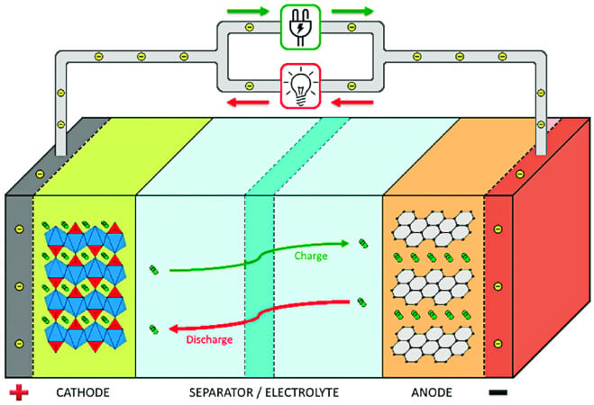
Figure 3. Schematic representation of a Li-ion battery and its operation. Image used courtesy of ResearchGate

 

In this diagram, as the electrons pass through the external circuit powering the load, the lithium ions pass through the separator membrane and electrolyte and reach the anode or cathode, depending on whether the battery is charged or discharged. The electrochemical model discussed earlier uses the chemical potential from the reversible reaction to estimate the state of charge and health. However, it has two limitations:

1. The state parameters are not uniform across the length of the cell

2. The chemical reactions are governed by multiple higher-order partial differential equations that require complex computations and have a high computing power burden

Recently, some models that use the particulate nature of the lithium ions and their physical diffusion across the electrolyte have been introduced to explain how an electric potential develops or changes across a cell.

The commonly used approaches for physics-based models are:

1. SPM or single particle model: This model treats each cell electrode as a single particle.

a. It disregards the gradients in the electrolyte concentration and considers it homogenous.

b. The electrode is considered a single uniform sphere.

c. This allows the current flux to be uniform across its surface.

With this simplified model, it is possible to calculate the voltage, current density, SEI layer, or the passivation layer development and degradation of the electrodes at low discharge rates. In addition, the particle kinetics of the electrochemical reactions to derive the electric potential are described by the Buttler-Volmer equation. Discussing the mechanics of this is beyond the scope of the article. However, it can be concluded that the SPM can be used to predict the state of charge or state of health of a cell. However, the model trades computational simplicity for accuracy. The native accuracy of this model is quite low, and the model gives unreliable results at high discharge rates due to localization charge concentration gradients.

2. P2D or pseudo-two-dimensional model: This model was developed to overcome the limitations of the single particle model.

The model is represented in Figure 4.

 

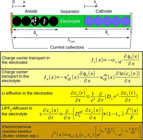
Figure 4. P2D battery model and its equations. Image used courtesy of ResearchGate

 

The model utilizes two independent spatial variables, ‘x’ to track concentration gradients along the length or thickness of the cell and ‘r’ to track the radial concentration in the solid electrode particles. The diagram indicates that the charge carrier concentration and diffusion are tracked in the electrode and the electrolyte. Finally, the reaction kinetics are calculated using the Butler-Volmer equation. It estimates the overpotential based on charge diffusion in solid and liquid phases. It can offer better accuracy compared to the single particle model. While this model has the potential for accuracy, it depends on the manufacturing chemistry and requires extensive collaboration with cell manufacturers for an accurate prediction. This is especially important since the model uses electrolyte and membrane/particulate diffusion modeling to predict the voltage at different loading scenarios. In many cases, manufacturers of cells are not willing to share specifics of cell composition and construction.

It is also extremely intensive computationally and, hence, is not ideal for the low power requirements imposed by battery-powered fuel gauges. For example, if we were to use 20 radial nodes, 50 electrode nodes, and 25 separator nodes, more than 2500 partial differential equations (PDE) must be solved to get the electric potential. After all, a fuel gauge is also powered by the battery it is attached to and needs to consume as little power as possible.

 

Alternative Modeling

Because of the complexities of modeling cells and the computational requirements imposed by the cell models, alternative approaches are needed to develop low-power BMS algorithms that can offer acceptable real-time accuracy and power consumption. To this end, the lookup table method is used along with coulomb counting to monitor cells.

The lookup table contains the open circuit battery voltage at different depths of discharge. It provides a static reference of the relaxed state of the battery with respect to capacity. It can be used as an analog of the state of charge or the remaining capacity related to the nominal battery capacity.

This can provide a known state to calculate the unloaded voltage given a loaded voltage curve. Based on the OCV, the battery's internal impedance can be calculated at various states of charge to provide a base model for a new battery. When used with coulomb counting with a battery of known capacity, this can be used to closely estimate the state of charge of a battery under a given discharge condition.

The model can be expanded to use multiple discharge rates to maintain relative accuracy across multiple discharge rates and temperatures. Temperature compensation is typically done using a slow-moving and a fast-moving exponential stochastic. The slow-moving stochastic improves accuracy across a full discharge cycle, while the fast stochastic can predict how self-heating affects the discharge capacity in a short time frame. The advantage of this 2-parameter approach is that the self-heating can be incorporated as an input into the longer time frame of a full cycle to improve accuracy further.

The current market space for fuel gauges is dominated by the equivalent circuit model used in tandem with the lookup table and coulomb counting. It has been proven to demonstrate acceptable levels of accuracy depending on the model fidelity and depth of data collected. 

The 2R2C battery model has been successfully implemented in various applications ranging from consumer-grade to industrial and automotive sectors.

Part 3 in this series will discuss how this model is used to develop a robust solution using Qorvo’s BMS products.