 Facebook
 Google
 GitHub
 Linkedin
How To Calculate Power Factor Correction
Sinusoidal Steady State Power
As you now know, reactive components can cause a circuit’s power factor to deviate from the ideal value of 1. However, a technique known as power factor correction allows us to modify a system such that it requires less reactive power yet continues to provide the necessary functionality.
A common form of power factor correction is the use of parallel capacitance to counteract the effect of inductive loads such as motors. In this page we’ll work through an example of this type of power factor correction.
Reactive power (denoted by Q) is an important concept in the context of power factor correction. In our example, the power factor will be equal to 1 if the magnitude of the reactive power due to the added capacitance (|QC|) is equal to the reactive power due to the circuit’s inductance (QL). This problem would be easier to solve if we knew the inductance, but let’s imagine that the reactive devices in the system don’t come with inductance specifications.
Step 1: Create the Impedance Triangle
Our example system is equivalent to the following circuit:
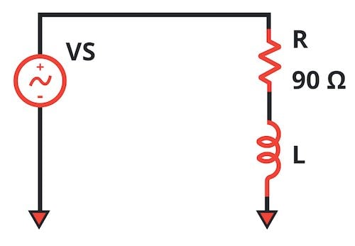
Figure 1. The system before power factor correction
The source is a typical 60 Hz, 115 VRMS supply voltage (the corresponding peak value is 163 V). We know that the resistance in the circuit is 90 Ω. As mentioned above, we don’t know the value of the inductance. After measuring the voltage and current, we find that there is a phase difference of 30°.
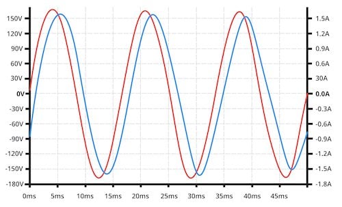
Figure 2. Measured current and voltage for the circuit shown in Figure 1. The orange trace is the source voltage, and the blue trace is the current supplied by the source.
At this point we have the information that we need to calculate the circuit’s reactance. We’ll use the impedance triangle; the horizontal side of the triangle is the resistance, and the angle between the horizontal side and the hypotenuse is the same as the phase difference between voltage and current.
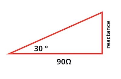
Figure 3. The impedance triangle for the circuit shown in Figure 1.
To calculate the reactance, we use the following equation:

Thus, the reactance of the circuit is 51.96 Ω.
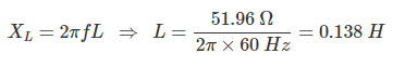
Step 2: Calculate Inductance and Capacitance
Before we determine the amount of capacitance needed to perform power factor correction, let’s find the circuit’s inductance. This information will be useful later when we perform simulations to verify our results. We’ve learned that the impedance of an inductor is equal to jωL; reactance (denoted by X) is simply the imaginary part of impedance, so the reactance of an inductor is XL = ωL = 2πfL.
The impedance of a capacitor is –j/(ωC), and thus XC = –1/(2πfC). As mentioned above, to achieve power factor correction, the magnitude of the reactive power created by the parallel capacitor must be equal to the reactive power created by the inductance.
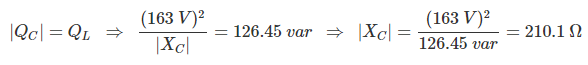
Our measurements indicated that the current supplied by the source, and hence the current through the inductor, has a peak value of approximately 1.56 A. Thus,

The voltage across the capacitor is equal to the source voltage, so we can find the required capacitive reactance as follows:
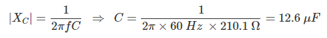
Now we calculate the power-factor-correction capacitance from the capacitive reactance:
Step 3: Verify the Results
Our power-factor-corrected system is equivalent to the following circuit:
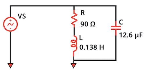
Figure 4. We’ve added a power-factor-correction capacitor in parallel with the original circuit.
If we simulate this circuit, we see that the voltage and current are now in phase, which is exactly what we expect when a system has a power factor of 1.
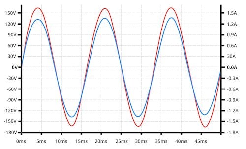
Figure 5. The system’s voltage (the orange trace) and current (the blue trace) are now in phase.
Review and Moving Forward
We’ve explored power factor correction by means of an example. In the next page, we’ll look at a fundamental and extremely common component in power systems, namely, the transformer.