Estimating Virtual Semiconductor Diode Temperature Using Dynamic Thermal Impedance Curves

In applications like switched-mode power supplies, semiconductor devices often run in pulsed mode, not continuous waves. These devices might never reach a stable operating point, making steady-state thermal resistance unsuitable for accurate thermal modeling.

 

Dynamic Thermal Impedance

Dynamic thermal impedance (Z_th) describes time-based heat transfer involving thermal resistance and capacitances during transient processes. Using the electrical analogy, these capacitances need to ‘charge up’ before heat disperses (illustrated for a diode in a surface-mounted SMD package thermal system in Figure 1a). Dynamic thermal resistance measures transient heat flow between two points, A and B, due to temperature differences. Z_th is also influenced by the applied signal pulse:

\[Z_{th(A-B)}(t_{pulse})=\frac{\partial T}{\partial P}|t=t_{pulse}\]

Z_th values, usually shown as curves in a diode’s datasheet, aid in calculating diode heating as a thermal system in pulsed scenarios. Yet, the calculation should also consider the signal’s pulse width and duty cycle.

 

Image used courtesy of Freepik

 

Foster and Cauer Modeling

The dynamic thermal behavior of semiconductor devices can be simulated using resistance-capacitance (RC) thermal networks known as Foster and Cauer models. Derived from heating curves, these RC models describe dynamic thermal impedance, such as for Nexperia’s PMEG050T150EIPD Schottky diode (Figure 1b). They capture the device's thermal response to transient power pulses by measuring power losses during various time spans equilibrium (steady-state). Here, Z_th levels off, aligning with R_th. This also highlights thermal inertia—material temperature changes aren’t immediate, enabling short bursts of high power. The figure presents Z_th curves for varied-duty repetitive pulses, indicating extra temperature elevation from RMS power dispersion.

 

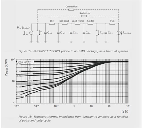
Image used courtesy of Bodo’s Power Systems [PDF]

 

How to Calculate a Rise in Junction Temperature

To determine junction temperature rise in a semiconductor device with a single active area (heat source at the junction), knowing the power and duration of a signal pulse is crucial. For square-wave power pulses, dynamic thermal impedance can be directly read from the Z_th chart. The temperature increase at the junction results from the product of this value and signal power. Alternatively, for constant power, steady-state thermal impedance R_th suffices, with temperature rise as the product of signal power and R_th.

For transient pulses (sinusoidal or pulse), calculating junction temperature rise is intricate. The mathematically accurate method involves using a convolution integral. This integrates power pulse and Z_th curve functions over time to yield the temperature profile after an event of duration τ.

\[\Delta T_{j}=\int^{\tau}_{0}P(t)\frac{dZ_{th}(\tau-t)}{dt}dt\]

However, this isn’t trivial since is not defined mathematically. Another option is approximating waveforms as a series of rectangular pulses through superposition. Yet, this method has drawbacks— complex waveforms demand diverse superpositions for accurate modeling. An alternative is presenting Z_th as an R_C thermal model, enabling junction temperature calculation via a SPICE simulator.

 

Equivalence Between Thermal and Electrical Parameters

Using Table 1, the values for a device’s thermal resistance and capacitance can be represented as equivalent electrical resistances and capacitances, respectively. In addition, representing current as power and voltage as temperature difference allows any thermal network to be treated as an electrical network.

 

Table 1. Electrical and thermal analogy for semiconductor devices.

Type	Resistance	Potential	Energy	Capacitance
Electrical (R=V/I)	R = ohmic resistance (Ohms)	V = electrical potential (Volts)	I = current (Amps)	C = capacitance (Farads)
Thermal (Rth = K/W)	Rth = Thermal resistance (K/W)	K = temperature difference (Kelvin)	W = dissipated power (Watts)	Cth = thermal capacitance (thermal mass)

 

A Foster model is developed by fitting a curve to Z_th, yielding a one-dimensional RC network. Yet, R and C values don’t correlate to physical device locations, preventing calculation from material constants. A drawback of the Foster RC model is its inability to divide or connect with other component models like heatsinks.

Foster RC models simplify expressing thermal impedance Z_th. For example, by measuring a heating (or cooling) curve for a device and generating a Z_th profile, the following equation can be used to create a ‘fitted’ curve, like that shown in Figure 2b:

\[Z_{th}(t)=\sum\limits{^{n}_{i=1}}\,Ri\times\Big(1-e^{-\frac{t}{\tau_{i}}}\Big)where\,\tau_{i}=R_{i}\times C_{i}\]

 

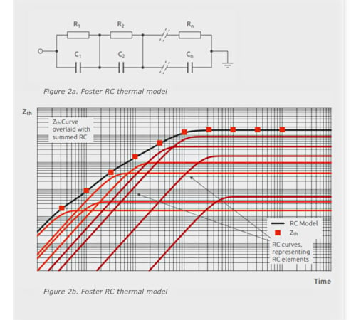
Image used courtesy of Bodo’s Power Systems [PDF]

 

Thermal resistances (Ri) and capacitances (Ci) form the basis of a thermal network model. By optimizing parameters in the analytical expression, the transient system response can match the time response through a least-squares curve-fitting algorithm. Foster models lack tangible significance, as node-to-node heat capacitances aren’t real. However, a Foster model can transform into its Cauer equivalent via a mathematical shift. An n-stage Cauer model is derived from an n-stage Foster model to equivalently represent thermal performance. Similar to Foster, Cauer models (Figure 3a) consist of an RC network, but with all thermal capacitances linked to thermal ground (ambient temperature). Unlike Foster, Cauer’s nodes hold physical meaning, enabling internal semiconductor layer temperature calculation.

 

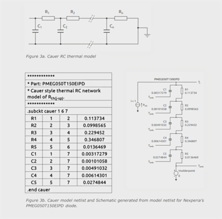
Image used courtesy of Bodo’s Power Systems [PDF]

 

While Foster and Cauer models are equivalent representations of a device’s thermal behavior, Cauer models are more representative of the physical structure of the device, so these are used in the following sections. A netlist for a Cauer network can be used to create a SPICE schematic (Figure 3b).

Pin 1 in the netlist is the junction temperature pin Tj in the schematic. Similarly, pins 6 and 7 represent the ambient temperature pin (Tamb). Only device pins 6 and 7 are connected to the ambient voltage source to simulate this thermal network. An added advantage of using the Cauer models is that they allow external networks to be connected, enabling the additional impact of PCB heating and heatsinks to be analyzed. To do this, pin 7 must be connected to the ambient temperature, and pin 6 to the first pin of the external Cauer network. For correct results, the termination pin of the external Cauer network must be connected to the ambient source.

 

Setting up a Thermal SPICE Simulation

The following steps are used to prepare and perform a SPICE simulation of the thermal network:

1. Set up the R_C thermal model of PMEG050T150EIPD in SPICE.

2. Set the value of voltage source V_solderpoint = 0, which is the value of T_sp.

3. Set the value of the current source P_tot = 1.

4. Create a simulation profile and set the run time to 100 ms.

5. Run the simulation.

6. Plot the voltage at node T_j.

The simulation result in Figure 4 shows the junction temperature (voltage at T_j), which is also the thermal impedance of the PMEG050T150EIPD.

From this screen plot, the values of Z_th at different times can be read using cursors in a SPICE waveform display. The value of the current source in this example is set to 1 A to represent 1 W of power being dissipated in the diode. This can be easily modified for any power profile. The simulation duration can also be changed to represent a range of square power pulses. The SPICE simulation can also investigate the temperature for internal device junctions.

 

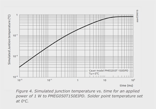
Image used courtesy of Bodo’s Power Systems [PDF]

 

Dynamic Thermal Impedance Summary

Dynamic thermal impedance (Z_th) stands as a comprehensive framework encompassing heat transfer nuances over time, integrating both thermal resistances and capacitances pertinent to transient processes. Contrastingly, conventional steady-state models falter in accurately characterizing device thermal behavior under pulsed applications. Enter Z_th curves, providing a remedy by offering a more faithful representation. This article has elucidated the theoretical foundation of this approach and substantiated its efficacy through a successful simulation of diode thermal behavior. Z_th curves thus emerge as a pivotal tool, enabling precise comprehension and projection of dynamic thermal operations.

 

This article originally appeared in Bodo’s Power Systems [PDF] magazine.